The CloudLab Manual
CloudLab is a "meta-cloud"—
The current CloudLab deployment consists of more than 33,000 cores in over 1800 allocatable nodes distributed across three sites at the University of Wisconsin, Clemson University, and the University of Utah. CloudLab interoperates with existing testbeds including GENI and Emulab, to take advantage of hardware at dozens of sites around the world.
The control software for CloudLab is open source, and is built on the foundation established for Emulab, GENI, and Apt. Pointers to the details of this control system can be found on CloudLab’s technology page.
1 Getting Started
This chapter will walk you through a simple experiment on CloudLab and introduce you to some of its basic concepts.
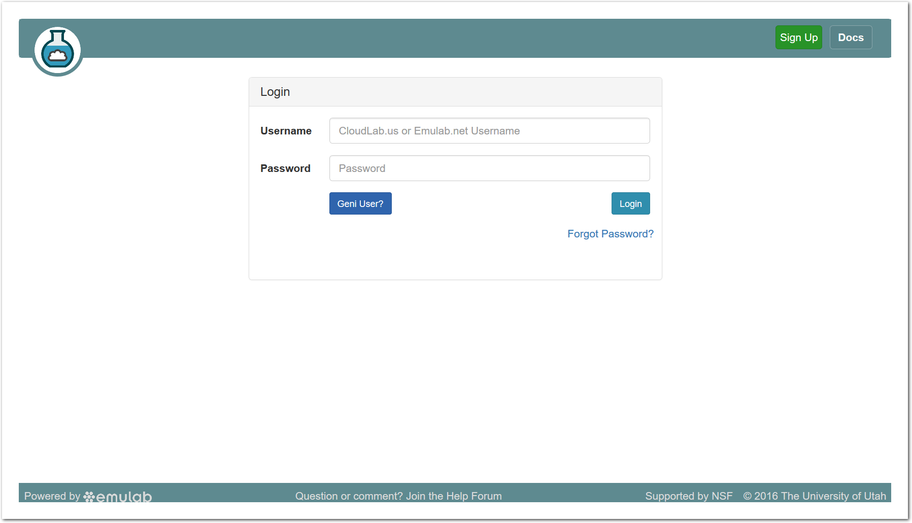
Start by pointing your browser at https://www.cloudlab.us/.
- Log inYou’ll need an account to use CloudLab. If you already have an account on Emulab.net, you may use that username and password. Or, if you have an account at the GENI portal, you may use the “GENI User” button to log in using that account. If not, you can apply to start a new project at https://www.cloudlab.us/signup.php and taking the "Start New Project" option. See the chapter about CloudLab users for more details about user accounts.
- Start ExperimentFrom the top menu, click “Experiments” and then “Start Experiment” to begin.
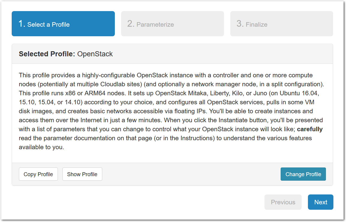
- Experiment WizardExperiments must be configured before they can be instantiated. A short wizard guides you through the process. The first step is to pick a profile for your experiment. A profile describes a set of resources (both hardware and software) that will be used to start your experiment. On the hardware side, the profile will control whether you get virtual machines or physical ones, how many there are, and what the network between them looks like. On the software side, the profile specifies the operating system and installed software.Profiles come from two sources. Some of them are provided by CloudLab itself, and provide standard installation of popular operating systems, software stacks, etc. Others are created by other researchers and may contain research software, artifacts and data used to gather published results, etc. Profiles represent a powerful way to enable repeatable research.Clicking the “Change Profile” button will let you select the profile that your experiment will be built from.
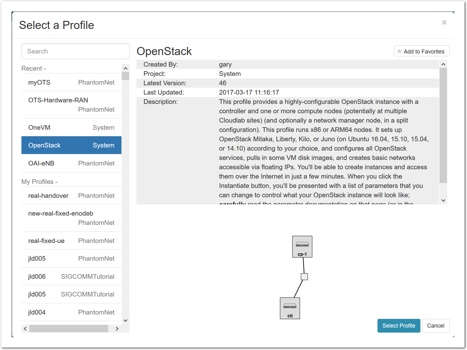
- Select a profileOn the left side is the profile selector which lists the profiles you can choose. The list contains both globally accessible profiles and profiles accessible to the projects you are part of.The large display in this dialog box shows the network topology of the profile, and a short description sits below the topology view.The OpenStack profile will give you a small OpenStack installation with one master node and one compute node. It provides a simple example of how complex software stacks can be packaged up within CloudLab. If you’d prefer to start from bare metal, look for one of the profiles that installs a stock operating system on physical machines.
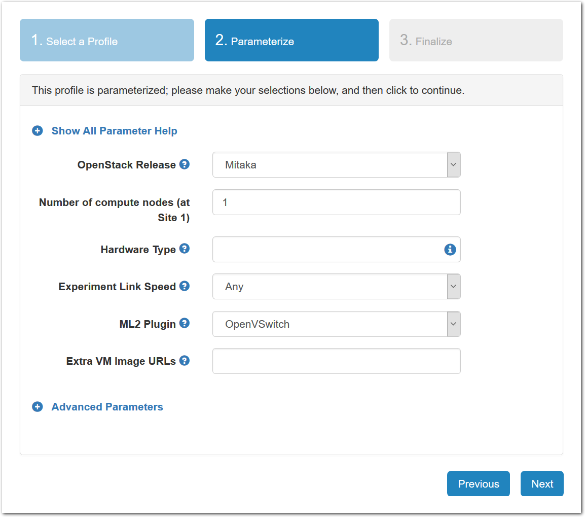
- Choose ParametersSome profiles are simple and provide the same topology every time they are instantiated. But others, like the OpenStack profile, are parameterized and allow users to make choices about how they are instantiated. The OpenStack profile allows you to pick the number of compute nodes, the hardware to use, and many more options. The creator of the profile chooses which options to allow and provides information on what those options mean. Just mouse over a blue ’?’ to see a description of an option. For now, stick with the default options and click “Next” to continue.
- Pick a clusterCloudLab can instantiate profiles on several different backend clusters. The cluster selector is located right above the “Create” button; the the cluster most suited to the profile you’ve chosen will be selected by default.
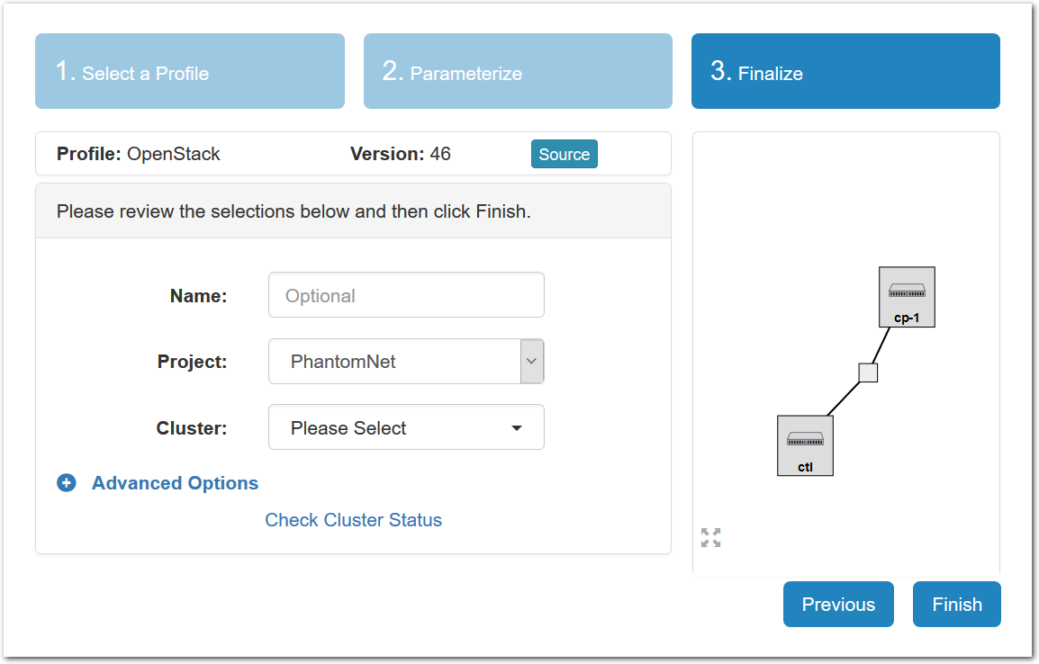
- Click Create!When you click the “Create” button, CloudLab will start preparing your experiment by selecting nodes, installing software, etc. as described in the profile. What’s going on behind the scenes is that on one (or more) of the machines in one of the CloudLab clusters, a disk is being imaged, VMs and/or physical machines booted, accounts created for you, etc. This process usually takes a couple of minutes.

- Use your experimentWhen your experiment is ready to use, the progress bar will be complete, and you’ll be given a lot of new options at the bottom of the screen.
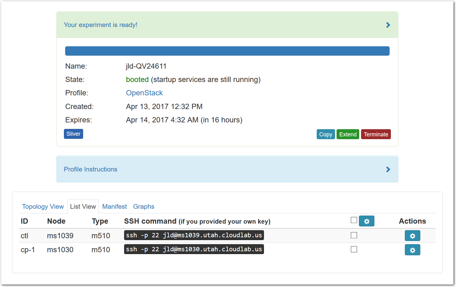 The “Topology View” shows the network topology of your experiment (which may be as simple as a single node). Clicking on a node in this view brings up a terminal in your browser that gives you a shell on the node. The “List View” lists all nodes in the topology, and in addition to the in-browser shell, gives you the command to ssh login to the node (if you provided a public key). The “Manifest” tab shows you the technical details of the resources allocated to your experiment. Any open terminals you have to the nodes show up as tabs on this page.Clicking on the “Profile Instructions” link (if present) will show instructions provided by the profile’s creator regarding its use.Your experiment is yours alone, and you have full “root” access (via the sudo command). No one else has access to the nodes in your experiment, and you may do anything at all inside of it, up to and including making radical changes to the operating system itself. We’ll clean it all up when you’re done!If you used our default OpenStack profile, the instructions will contain a link to the OpenStack web interface. The instructions will also give you a username and password to use.
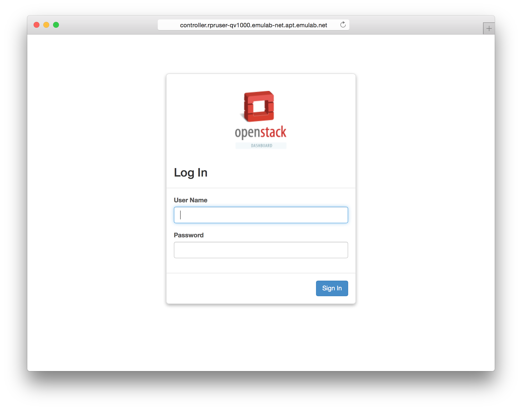 Since you gave CloudLab an ssh public key as part of account creation, you can log in using the ssh client on your laptop or desktop. The contoller node is a good place to start, since you can poke around with the OpenStack admin commands. Go to the "list view" on the experiment page to get a full command line for the ssh command.
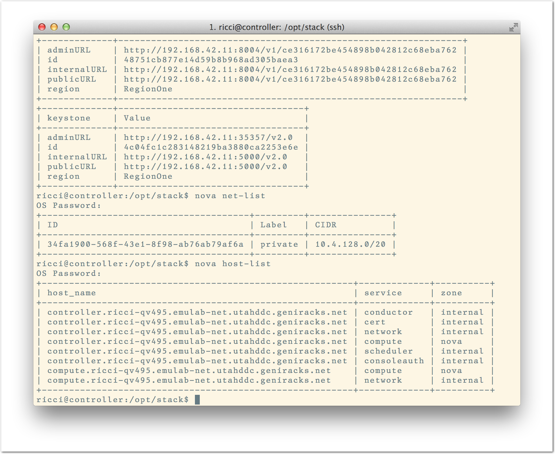 Your experiment will terminate automatically after a few hours. When the experiment terminates, you will lose anything on disk on the nodes, so be sure to copy off anything important early and often. You can use the “Extend” button to submit a request to hold it longer, or the “Terminate” button to end it early.
1.1 Next Steps
Try a profile that runs bare metal and set up a cloud stack yourself
Making your own profiles is easy: see the chapter on profile creation for instructions.
If you need help, or have questions or comments about CloudLab’s features, contact us!
2 CloudLab Users
Registering for an account is quick and easy. Registering doesn’t cost anything, it’s simply for accountability. We just ask that if you’re going to use CloudLab for anything other than light use, you tell us a bit more about who you are and what you want to use CloudLab for.
Users in CloudLab are grouped into projects: a project is a (loosely-defined) group of people working together on some common goal, whether that be a research project, a class, etc. CloudLab places a lot of trust on project leaders, including the ability to authorize others to use the CloudLab. We therefore require that project leaders be faculty, senior research staff, or others who are relatively senior positions.
2.1 Register for an Account
To get an account on CloudLab, you either join an existing project or create a new one. In general, if you are a student, you should join a project led by a faculty member with whom you’re working.
If you already have an account on
Emulab.net, you don’t need to sign
up for a new account on CloudLab—
2.1.1 Join an existing project
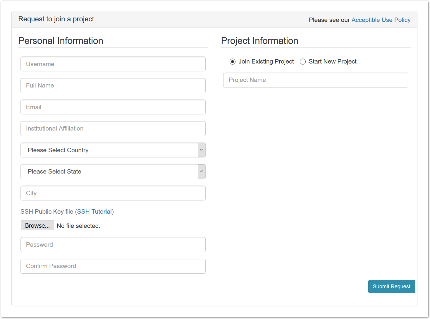
To join an existing project, simply use the “Sign Up” button found on every CloudLab page. The form will ask you a few basic questions about yourself and the institution you’re affiliated with.
An SSH public key is required; if you’re unfamiliar with creating and using ssh keypairs, we recommend taking a look at the first few steps in GitHub’s guide to generating SSH keys. (Obviously, the steps about how to upload the keypair into GitHub don’t apply to CloudLab.)
CloudLab will send you email to confirm your address—
watch for it (it might end up in your spam folder), as your request won’t be processed until you’ve confirmed your address.
2.1.2 Create a new project
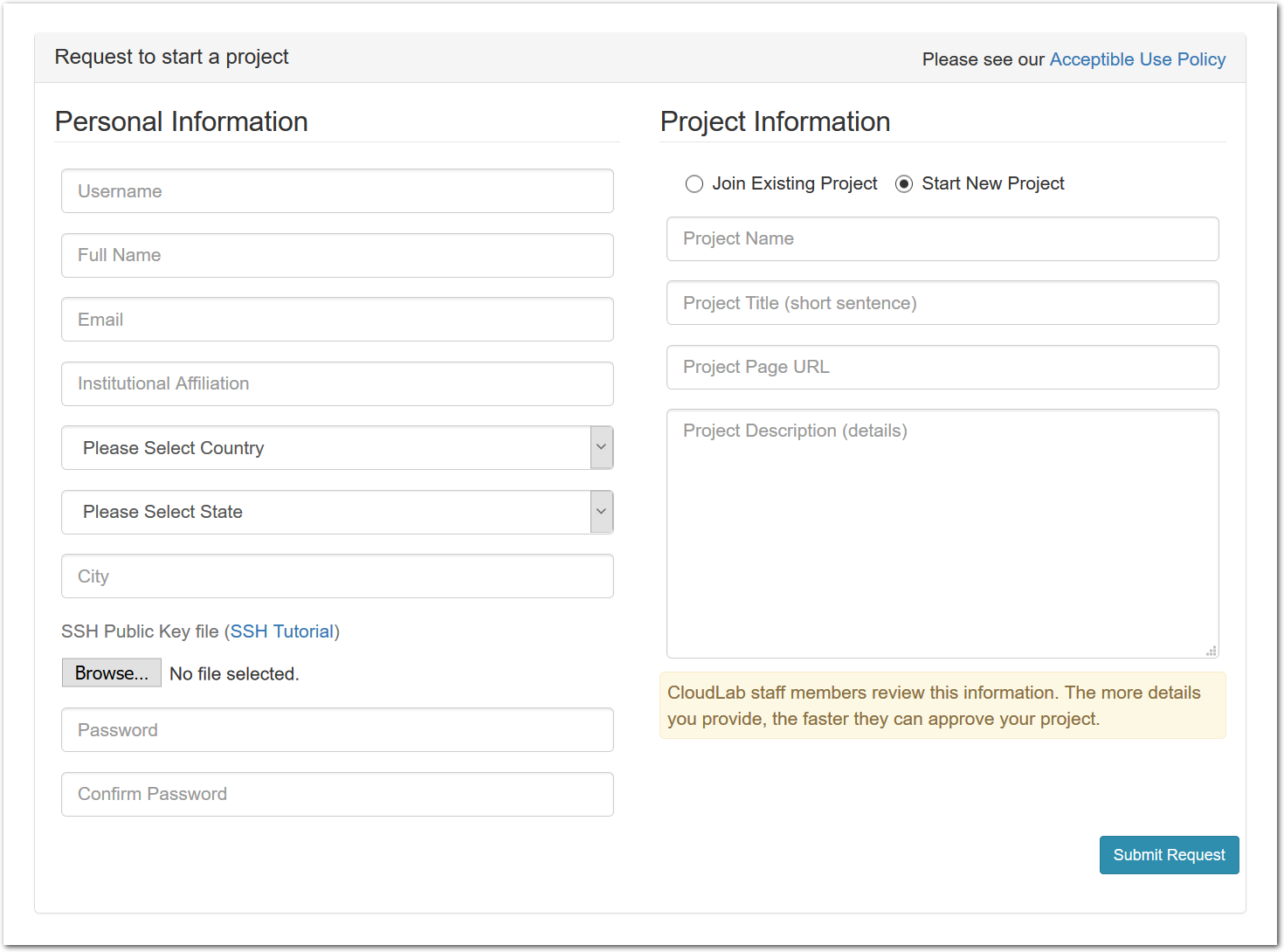
You should only start a new project if you are a faculty member, senior research staff, or in some other senior position. Students should ask their advisor or course instructor to create a new project.
To start a new project, use the “Sign Up” button found on every CloudLab page. In addition to basic information about yourself, the form will ask you a few questions about how you intend to use CloudLab. The application will be reviewed by our staff, so please provide enough information for us to understand the research or educational value of your project. The review process may take a few days, and you will receive mail informing you of the outcome.
Every person working in your project needs to have their own account. You get to approve these additional users yourself (you will receive email when anyone applies to join.) It is common, for example, for a faculty member to create a project which is primarily used by his or her students, who are the ones who run experiments. We still require that the project leader be the faculty member, as we require that there is someone in a position of authority we can contact if there are questions about the activities of the project.
Note that projects in CloudLab are publicly-listed: a page that allows users to see a list of all projects and search through them does not exist yet, but it will in the future.
2.1.3 Setting up SSH access
The first step to setting up ssh access to CloudLab is to generate an ssh key pair.
**For Windows users:**
A good option for a Windows ssh client is to make use of putty:
To generate and manage ssh keys with putty:
https://www.ssh.com/ssh/putty/windows/puttygen
**For Linux and Mac OS users:**
To generate and manage ssh keys:
https://www.ssh.com/ssh/keygen/
Once you have generated an ssh key pair, you need to upload the public key into the CloudLab portal:
Log into the CloudLab portal. Once you are logged in: Click on your username (top right), select "Manage SSH keys" and follow the prompts to load the ssh public key.
The next time you instantiate an experiment, your ssh public key will be loaded onto all (ssh capable) nodes in your experiment, allowing direct access to these nodes using an ssh client.
2.1.4 Setting up X11
Experiment based graphical user interface (GUI) interaction on CloudLab often require X windows, so you might find it useful to have an X-server running on the laptop/desktop you use to access resources on CloudLab.
**For Windows users:**
Various options are available, for example:
https://sourceforge.net/projects/vcxsrv/
**For Mac OS users:**
3 CloudLab and Repeatable Research
One of CloudLab’s key goals is to enable repeatable research—
CloudLab is designed as a scientific instrument. It gives full visibility into every aspect of the facility, and it’s designed to minimize the impact that simultaneous slices have on each other. This means that researchers using CloudLab can fully understand why their systems behave the way they do, and can have confidence that the results that they gather are not artifacts of competition for shared hardware resources. CloudLab profiles can also be published, giving other researchers the exact same environment—hardware and software—on which to repeat experiments and compare results.
CloudLab gives exclusive access to compute resources to one experiment at a time. (That experiment may involve re-exporting those resources to other users, for example, by running cloud services.) Storage resources attached to them (eg. local disk) are also used by a single experiment at a time, and it is possible to run experiments that have exclusive access to switches.
3.1 CloudLab For Artifact Evaluation
CloudLab is an ideal environment for artifact evaluation: it provides a way for authors to define an environment in which they know their experiments will work, and a way for AEC members to get access to large collections of computing hardware without having to own that hardware themselves or pay for a commercial cloud environment.
In this section, we offer advice to authors of artifacts, AEC chairs, and the members of AECs.
3.1.1 For Authors
The best way to give evaluators a predictable environment is to provide a link to a profile that is suitable for running your artifact. This could be one of our standard profiles, or one that you make yourself. Either way, you can be sure of the environment they will get so that you do not have to worry about hardware differences, software versions, etc. This profile may be simple, giving them access to a single machine with a default OS, or may have multiple machines and/or use features such as disk images and startup scripts to manage dependencies and configuration so that the evaluators have minimal work to do.
On the page for each profile, there is a "share" button: this will provide you with the link you can give to evaluators. Because profiles are versioned, you can provide them with a link to either a specific version of the profile or to the profile in general (which will always point to the latest version). If you are using a profile that you made yourself, we recommend that you set the profile to be publicly available, though it is also possible to share private profiles (these use a link with a random identifier; anyone with the link can use the profile).
Evaluators will need to have a CloudLab account to use your profile. We do not recommend having them join your project (as this removes their anonymity) or giving them access to a running experiment (as this can be unnecessarily complex, and requires your experiment to remain instantiated for a potentially long period of time). Instead, we recommend that evaluators use accounts obtained as described below in the "AEC Chairs" and "AEC Members" sections. You may point them to this manual to explain the process if they are not familiar with it.
We recommend using a profile that specifies a specific hardware type so that you can ensure that evaluators are running on machines with the same type of performance, the same amount of memory, etc. We also recommend that you use a profile that specifies an explicit disk image(s) to use, even if that image is one of CloudLab’s default images. This way, even if CloudLab’s default changes, you can be assured that evaluators will continue to get the same one you used and will not run into any unexpected software version problems.
Because many artifacts are shared as git repositories, repo-based profiles can be a good way to package the profile with the rest of the artifact. In essence, any public git repo can be made into a profile by adding a profile.py script (which defines the profile using Describing a profile with python and geni-lib) to it. If you chose to do this, you will still provide the evaluators with a link to a profile to use: it will just be the case that the definition of this profile is contained within the same repository as the rest of your artifact. For an example of this, see the artifact repository for the OrderSage project.
3.1.2 For AEC Chairs
CloudLab can be a useful resource for AECs as a place with significant resources to run artifacts. It can be useful whether or not artifacts are submitted as CloudLab profiles (as described above): AEC members can get machines with a variety of hardware and popular OSes, and they have root access, so installing dependencies, etc. is straightforward. Many members of certain research communities will already have experience using CloudLab.
We recommend that AEC chairs start a project for the AEC; the CloudLab staff will review your project application, so make sure it is clear about which venue it is an AEC for. Once the project is approved, you will receive links that you can share with AEC members to join the project. Project leads approve members of their projects, so CloudLab staff will not be involved further in the process.
CloudLab can sometimes be quite busy, and resources (especially hardware with particularly valuable properties) can fill up. We recommend that you warn your AEC members to plan ahead and leave themselves plenty of time to make sure they can get the resources they need. The reservation system can be used to help get access to scarce resources.
3.1.3 For AEC Members
CloudLab can be a useful resource for AEC members whether or not artifacts are submitted as CloudLab profiles (as described above): AEC members can get machines with a variety of hardware and popular OSes, and they have root access, so installing dependencies, etc. is straightforward.
We recommend that AEC members join a project created specifically for the AEC. If your AEC chairs have not provided you with information about a CloudLab project for the AEC, we recommend that you point them to the section above for instructions to create one.
If you already have an account on CloudLab, it is possible to be a member of multiple projects with the same account; simply log in to your existing account before applying to join the new project.
Since AECs frequently work on tight deadlines, and CloudLab has limited resources, we recommend planning ahead to make sure that you have enough time to obtain the resources you need and do the evaluation. If you are having trouble with the resources you need being unavailable, have a look at CloudLab’s reservation system.
4 Creating Profiles
In CloudLab, a profile captures an entire cloud environment—
When you create a new profile, you are creating a new geni-lib python script, and, often, creating one or more disk images that are referenced by that script. When someone uses your profile, they will get their own experiment that boots up the resources (virtual or physical) described by the profile script.
To create profiles, you must be a registered user.
When you create a new profile, you can provide the geni-lib python script to CloudLab in one of two ways. First, you can upload it as a single file, allowing CloudLab to manage its storage, and upload a modified version or edit it in the CloudLab code editor when you want to create a new version. Second, you can use CloudLab’s repository-based profile feature, in which you provide a git repository URL containing the geni-lib python script as a profile.py file in the top-level directory of the repository. This allows you to control versioning according to your git workflow and instantiate from branches. We discuss both of these modes in more detail in the following subsections.
4.1 Creating a profile from an existing one
The easiest way to create a new profile is by copying an existing one and customizing it to your needs. Your goal should be to choose the profile that is most similar to the one you want to build. Usually, this will be one of our facility-provided profiles with a generic installation of Linux.
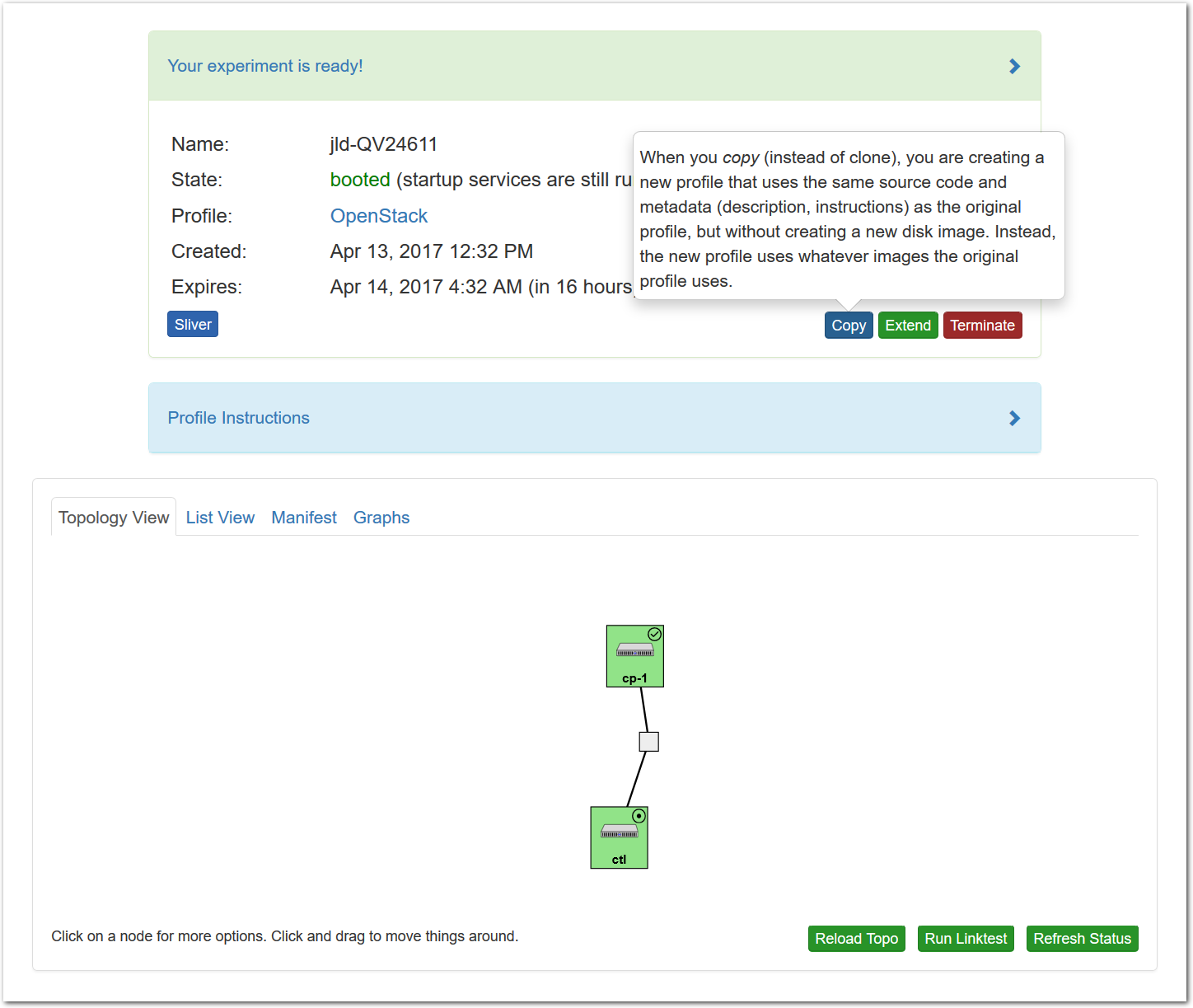
When you copy a profile, you are creating a new profile that is identical in every way to an existing profile. You may or may not have a running experiment using the source profile. And if you do have a running experiment, it does not impact the copy. After copying a profile, you can then modify it for your own use. And if you instantiate the copy, you can then take snapshots of disk images and use them in future version of your copy. You can copy any profile that you have access to.
4.1.1 Copying a Profile
- Choose a profileFind the profile you wish to copy using the “Start Experiment” selector. Then you can click “Show Profile” button, and click the “Copy” button on the resulting page to copy the profile directly; or you can instantiate the profile if you wish to create an experiment first. Both profiles themselves and active experiments can be copied.
- Copy the profile or experimentWhile logged in, both your experiment page and the show profile page will have a copy button. Clicking this button will create a profile based on that profile or experiment.This button only copies the geni-lib python script. No state in the active experiment is preserved.
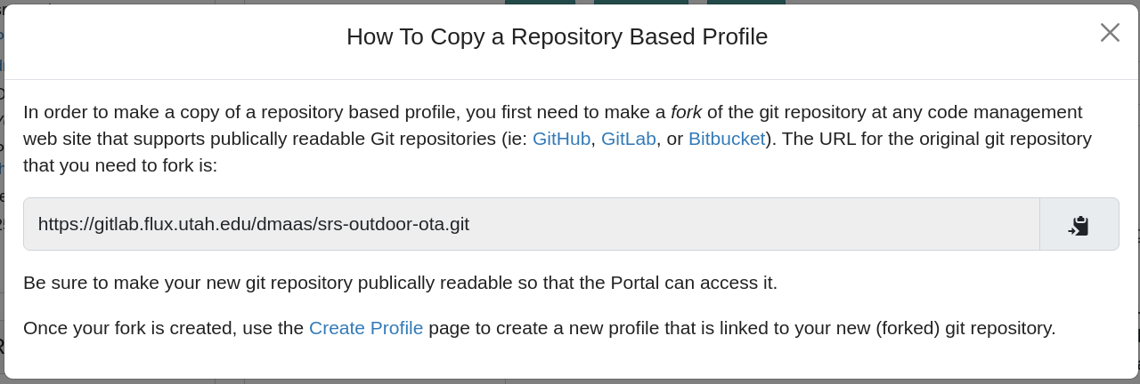
- Copying repository-based profilesNote: when you copy a repository-based profile, you will be instructed to first fork the git repository, and use that to create a new profile, as shown in the following screenshot. This is necessary because CloudLab does not act as a Git repository hosting provider, due to the potentially large size of code repositories with embedded profiles, and the fact that most repository owners prefer to store their code on Github or a private on-premises Git hosting solution.
- Create ProfileYou will be taken to a complete profile form and should fill it out as described below.
4.1.2 Creating the Profile
After copying a profile (see above) or selecting the menu option to create a new profile from scratch, you will need to fill out the profile creation form in order to complete the creation process.
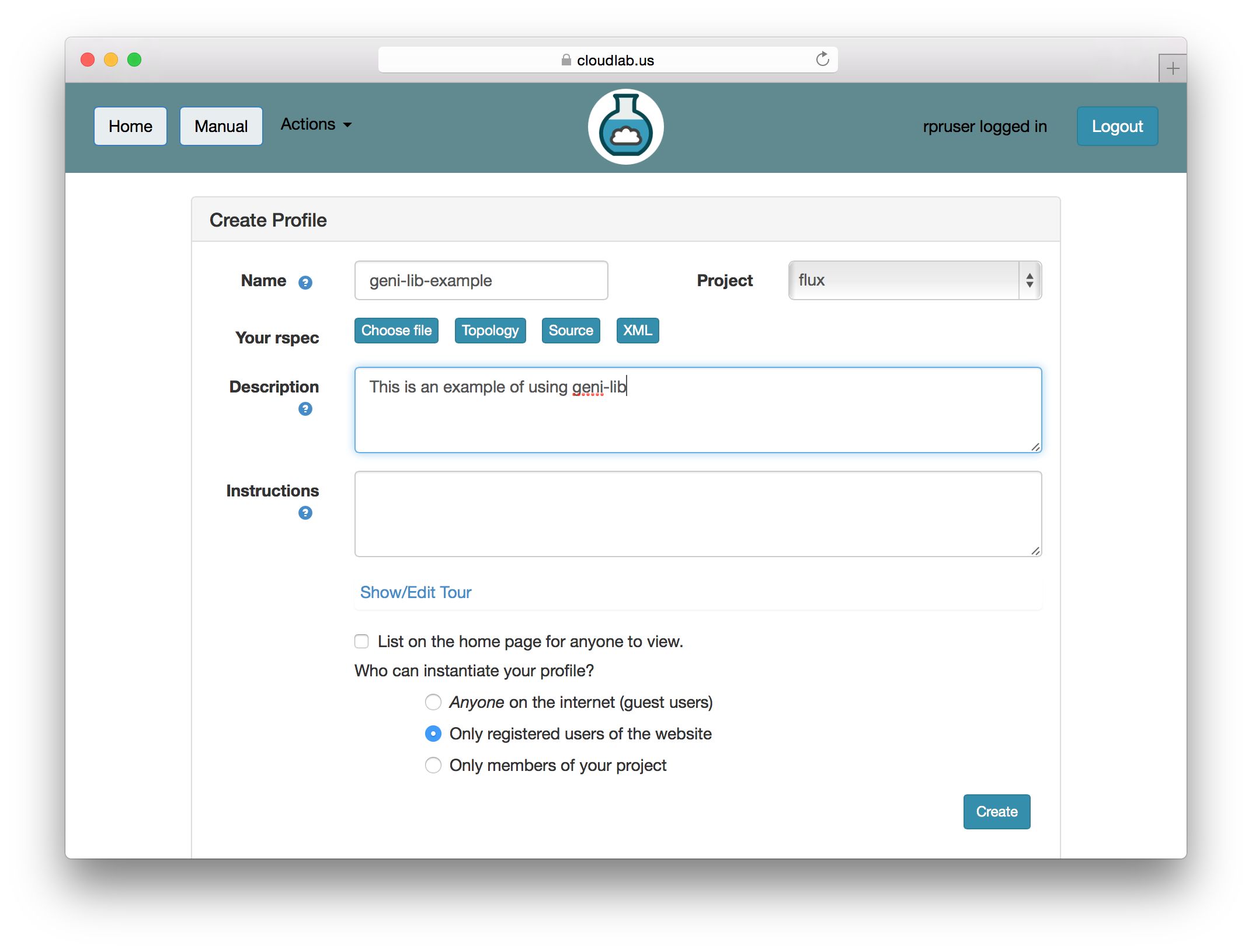
- Fill out information for the new profileAfter clicking on the “Copy” button, you will see a form that allows you to view and edit the basic information associated with your profile.
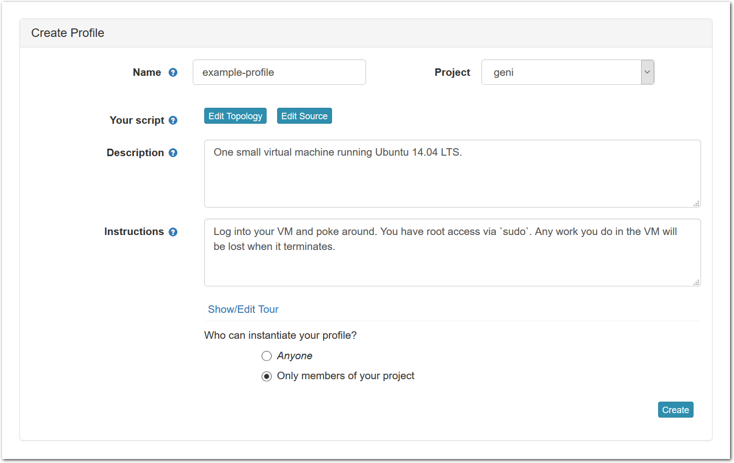 Each profile must be associated with a project. If you’re a member of more than one project, you’ll need to select which one you want the profile to belong to.Make sure to edit the profile’s Description and Instructions.The “Description” is the text that users will see when your profile is listed in CloudLab, when the user is selecting which profile to use. It is also displayed when following a direct link to your profile. It should give the reader a brief description of what they will get if they create an experiment with this profile. If the profile is associated with a paper or other publication, this is a good place to mention that. Markdown markup, including hyperlinks, are allowed in the profile description.The “Instructions” text is displayed on the experiment page after the user has created an experiment using the profile. This is a good place to tell them where the code and data can be found, what scripts they might want to run, etc. Again, Markdown is allowed.You may use template variables in your profile “Instructions” text to customize the instructions to an experiment. Currently, we support two kinds of template variables: host and password. Host variables will allow the Instructions template renderer to substitute a particular node’s FQDN—
recall that CloudLab FQDNs may be different for each experiment, since they contain both the experiment and project names as subdomains. For instance, if your profile includes a node named node-0, you could refer to its FQDN in the Instructions via {host-node-0}. You might use this to compose a URL to a service running on one of your nodes, e.g. for demos. Password variables allow you to expand specific random per-experiment passwords in the rendered instructions. If your profile includes a random password named perExptPassword, you can have it rendered in the generated Instructions via {password-perExptPassword}. The “Steps” section allows you to create a “tour” of your profile, which is displayed after a user creates an experiment with it. This feature is mostly useful if your profile contains more than one node, and you wish to explain to the user what the purpose of each node is.You have the option of making your profile usable to anyone, only registered CloudLab users, or members of your project. Regardless of the setting you chose here, CloudLab will also give you a direct link that you can use to share your profile with others of your choosing. - Test your profileIf you created your profile to capture an existing, manually configured experiment in a more reproducible manner, before terminating your experiment (or letting it expire), we strongly recommend testing out the new profile. If you elected to make it publicly visible, it will be listed in the profile selection dialog on the front page of https://www.cloudlab.us/. If not, you can instantiate it from the listing in your “My Profiles” page. If the profile will be used by guest users, we recommend testing it as one yourself: log out, and instantiate it using a different username (you will also have to use an alternate email address.)
- Share your profileNow that your profile is working, you can share it with others by sending them direct links, putting links on your webpage or in papers, etc. See “Sharing Profiles” for more details.
4.1.3 Updating a profile
You can update the metadata associated with a profile at any time by going to the “My Profiles” page and clicking on the name of the profile to go to the profile page. On this page, you can edit any of the text fields (Description, Instructions, etc.), change the permissions, etc.
If you need to update the contents of the disk image in the profile, simply create a new experiment from the profile. (You will only see this button on experiments created from profiles that you own.) Once your experiment is ready, you will see a “Create Disk Image” button on the experiment page. Log into your node, get the disk changed the way you want, and click the button. If your experiment includes multiple nodes, you will be given a dropdown to select from which node to capture the disk image. If you want to update the existing disk image the node is using, make sure to use the same name used in the profile, excluding the project name. (Note that disk images are captured into the same project in which the experiment is running.) If you use the same name, future experiments created from the profile will use the new image. However, if you want to create a new disk image, use a different disk image name, and after the image is successfully captured, edit your profile to reference the new disk image name.
As with creating a new profile, we recommend testing the profile before letting your experiment expire. If something goes wrong, we do keep one previous image file for each profile; currently, the only way to get access to this backup is to contact us.
4.2 Creating a profile with a GUI
CloudLab embeds the Jacks GUI for simple creation of small profiles. Jacks can be accessed by clicking the “topology” button on the profile creation or editing page. Jacks is designed to be simple, and to ensure that the topologies drawn can be instantiated on the hardware available. Thus, after making certain choices (such as picking an operating system image) you may find that other choices (such as the node type) become limited.
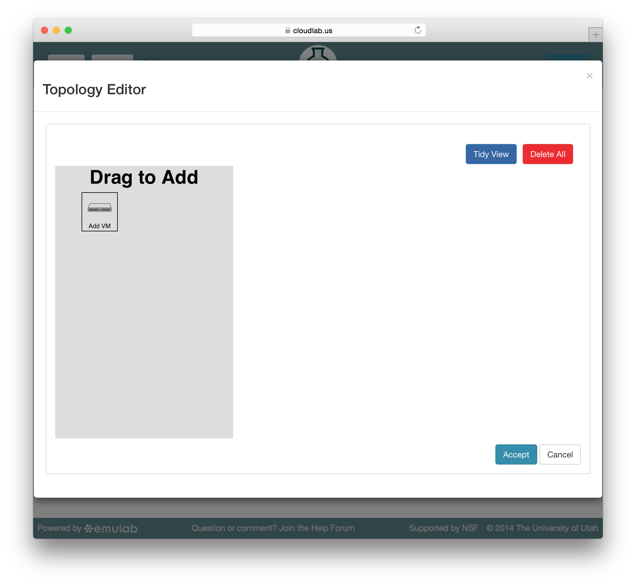
Jacks has a “palette” on the left side, giving the set of node types (such as physical or virtual machines) that are available. Dragging a node from this palette onto the larger canvas area on the right adds it to the topology. To create a link between nodes, move the mouse near the first node, and a small black line will appear. Click and drag to the second node to complete the link. To create a LAN (multi-endpoint link), create a link between two nodes, then drag links from other nodes to the small grey box that appears in the middle of the original link.
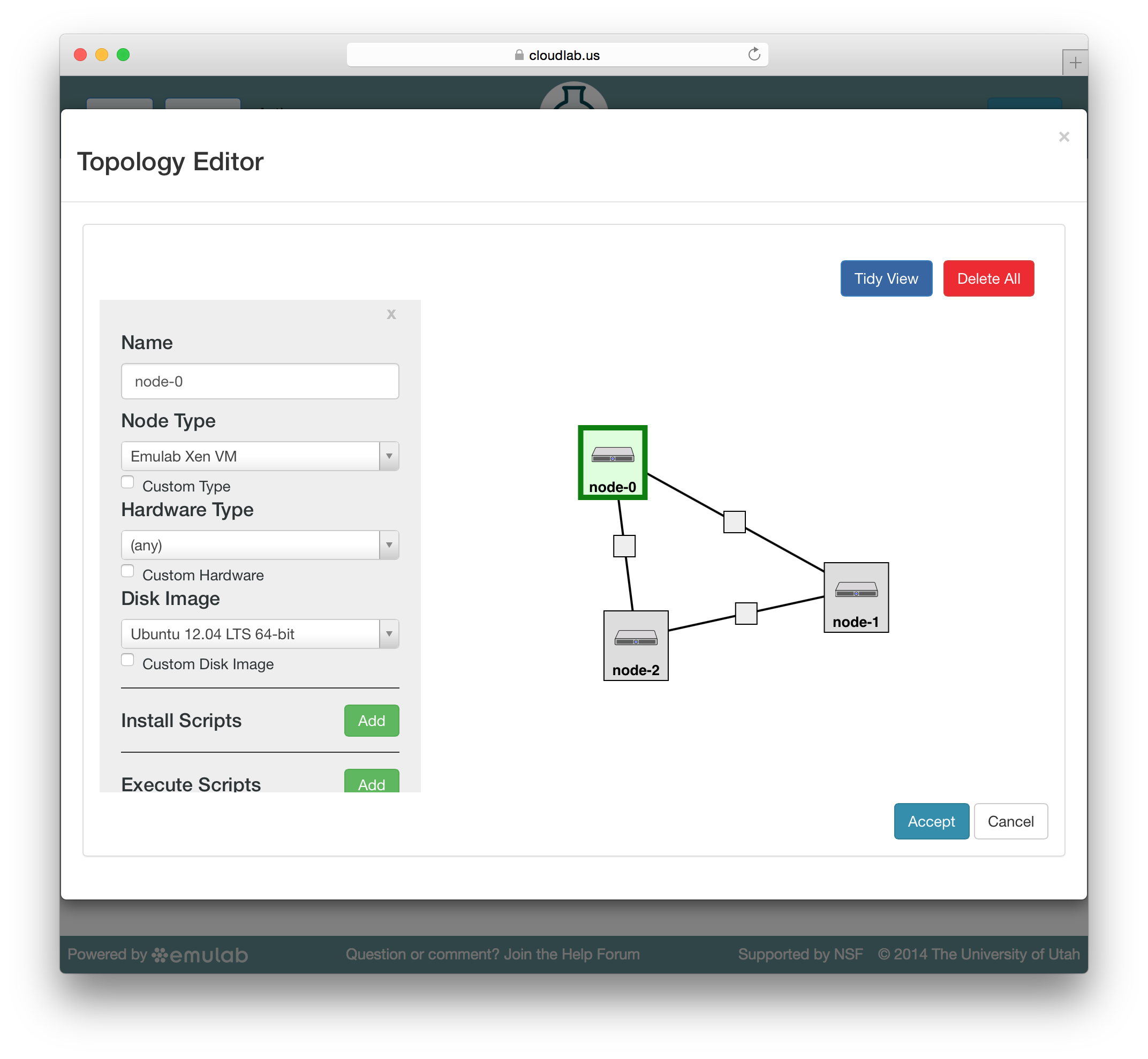
To edit the properties of a node or link, select it by clicking on its icon on the canvas. The panel on the left side will be replace by a property editor that will allow you to to set the disk image for the node, set commands to be run when the node boots, etc. To unselect the current node or link, and return to the palette on the left, simply click a blank area of the canvas.
4.3 Capturing Disk Images for Profiles
If you created a new profile by copying one of our standard or example
profiles, your profile is likely using a CloudLab-supported, standard disk
image. If you copied another user’s profile, you may instead be using a
custom disk image that the other user captured when they created their
profile. Depending on the nature of your profile, you may be satisfied to
continue using the original profile’s disk images, or you may prefer to
customize the disk images and persist changes of your own. Some profile
authors rely on CloudLab’s standard disk images, and customize these images
when the experiment boots via
startup scripts contained
in their profiles—
If you want to customize your copy of the profile and persist disk image changes, or ensure that your profile no longer depends on the disk images used in the original profile, you will want to create one or more custom disk images as used in the profile, and update the geni-lib python script in your copy of the profile to use the new image names:
- Create an experimentCreate an experiment using your copy of the original profile.
- Set up the node the way you want itLog into the node and install your software, datasets, packages, etc. Note the caveat below that any changes you make must remain outside of your home directory, and should not be tied to your user account.
- Capture a new disk imageWhile you are logged in, the experiment page for your active experiments will have a “Create Disk Image” button. Clicking this button will create a new disk image from one of the nodes in your running experiment. When customizing the image used by a profile that you do not own, you will need to create new image names, and update the geni-lib python script in your copy of the profile to use the new image names.
Capturing a disk image from an experiment can take a while, so we recommend that you extend your experiment before capturing the disk image, and contact us if you are worried your experiment might expire before you’re done creating your image. We also strongly recommend testing your profile fully before terminating the experiment you’re capturing the disk image from.
When capturing an image, your home directory is not included in the disk image snapshot! You will need to install your code and data elsewhere in the image. We recommend /local/. Keep in mind that others who use your profile are going to have their own accounts, so make sure that nothing in your image makes assumptions about the username, home directory, etc. of the user running it.
When capturing an image, be aware that only disk contents (not running process, etc.) are preserved, and as part of the creation process, your node(s) will first be rebooted in order to take consistent snapshots of the disk.
When copying a profile, remember that the disk images of a currently running experiment are not saved. If you want to customize the disk images using copy, you must copy the profile first, then instantiate your copy, then take snapshots of the modified disk image in your experiment.
4.4 Repository-Based Profiles
You can turn any public git repository (including those hosted on GitHub) into a CloudLab profile. Simply place a geni-lib script named profile.py into the top-level directory of your repository. When you create a new profile, you can provide the URL for your repository. The URL needs to be a http:// or https:// URL, and the CloudLab portal needs to be able to clone the repository without authentication.
Note that CloudLab is not a git hosting service; while we do keep a cache of your repository, we don’t guarantee that the profile will continue to work if the original repository becomes unavailable. We also have limits on the size of the repositories that we will clone.
When you instantiate a repository-based profile, the repository will be cloned into the directory /local/repository on all nodes in the experiment. This means that you can keep source code, startup scripts, etc. in your repository and reference them from profile.py. CloudLab sets the pull URL for all of these clones to be your “upstream” repository, and attempts to set a suitable push URL for (it assumes that the hosting service uses ssh for pushes, and uses the git@<hostname>:user/repo convention). As a result, git pull and git push should be connected to your repository.
There is an example repository on GitHub at https://github.com/emulab/my-profile; if you don’t already have a git repository created, a good way to get started is to fork this one and create a new profile pointing at your fork.
Pushing to your repository is still governed by the authentication and permissions of your git hosting service, so others using your profile will generally be unable to push to your repository.
4.4.1 Updating Repository-Based Profiles
By default, the CloudLab profile does not automatically update whenever you push to your upstream repository; this means that people instantiating your profile see the repository as it existed at the time CloudLab last pulled from it.
You can manually cause CloudLab to pull from your repository using the “Update” button on the profile management page.
You can also set up CloudLab to automatically pull from your repository whever it is updating. To do so, you will need to set up a “web hook” on the service that hosts your git repository. CloudLab currently supports webhooks for GitHub.com, BitBucket.org, and sites hosted using GitLab (including both GitLab.com and self-hosted GitLab installations.) See the “push URL” in the Repository Info panel on the left side of the profile page for the webhook URL, and use the “information” icon next to it to get specific instructions for setting up a webhook on each service. Once you have set the webhook up, every time you push to your repository, your hosting service will let CloudLab know that it should automatically initiate a pull. (This will not be instantaneous, but should complete quickly in most cases.)
4.4.2 Branches and Tags in Repository-Based Profiles
By default, repository-based profiles will be instantiated from the default branch of the repository; this is typically the main or master branch. At the bottom of the profile page, you will also find a list of all branches and tags in the repository, and can instantiate the version contained in any of them. Branches can be used for development work that is not yet ready to become the master (default) version of the profile, and tags can be used to mark specific versions of the profiles that were used for specific papers or course assignments, for example.
4.5 Creating a profile from scratch
CloudLab profiles are described by GENI RSpecs. You can create a profile directly from an RSpec by using the “Create Profile” option from the “Storage” menu. Note that you cannot edit the text fields until you upload an RSpec, as these fields edit (in-browser) fields in the RSpec.
4.6 Sharing Profiles
If you chose to make your profile publicly visible, it will show up in the main
“Select Profile” list on https://www.cloudlab.us/. CloudLab also gives you direct links to
your profiles so that you can share them with others, post them on your
website, publish them in papers, etc. The link can be found on the profile’s
detail page, which is linked for your “My Profiles” page. If you chose to
make your profile accessible to anyone, the link will take the form
https://www.cloudlab.us//p/<project-id>/<profile-id>. If you didn’t make the profile
public, the URL will have the form https://www.cloudlab.us//p/<UUID>, where
UUID is a 128-bit number so that the URL is not guessable. You can still
share this URLs with anyone you want to have access to the profile—
4.7 Versioned Profiles
Profiles are versioned to capture the evolution of a profile over time. When updating profiles, the result is be a new version that does not (entirely) replace the profile being updated.
When sharing a profile, you are given two links to share. One link will take the user to the most recent version of the profile that exists at the time they click the link. This is the most appropriate option in most cases. There is also a link that takes one to a specific version of the profile. This link is most useful for publication in papers or other cases in which reproducability with the exact same environment is a concnern.
5 Basic Concepts
This chapter covers the basic concepts that you’ll need to understand in order to use CloudLab.
5.1 Profiles
A profile encapsulates everything needed to run an experiment. It consists of two main parts: a description of the resources (hardware, storage, network, etc.) needed to run the experiment, and the software artifacts that run on those resources.
The resource specification is in the RSpec format. The RSpec describes an entire topology: this includes the nodes (hosts) that the software will run on, the storage that they are attached to, and the network that connects them. The nodes may be virtual machines or physical servers. The RSpec can specify the properties of these nodes, such as how much RAM they should have, how many cores, etc., or can directly reference a specific class of hardware available in one of CloudLab’s clusters. The network topology can include point to point links, LANs, etc. and may be either built from Ethernet or Infiniband.
The primary way that software is associated with a profile is through
disk images. A disk image (often just called an
“image”) is a block-level snapshot of the contents of a real or virtual
disk—
Profiles come from two sources: some are provided by CloudLab itself; these tend to be standard installations of popular operating systems and software stacks. Profiles may also be provided by CloudLab’s users, as a way for communities to share research artifacts.
5.1.1 On-demand Profiles
Profiles in CloudLab may be on-demand profiles, which means that they are designed to be instantiated for a relatively short period of time (hours or days). Each person instantiating the profile gets their own experiment, so everyone using the profile is doing so independently on their own set of resources.
5.1.2 Persistent Profiles
CloudLab also supports persistent profiles, which are longer-lived (weeks
or months) and are set up to be shared by multiple users. A persistent profile
can be thought of as a “testbed within a testbed”—
An instance of a cloud software stack, providing VMs to a large community
A cluster set up with a specific software stack for a class
A persistent instance of a database or other resource used by a large research community
Machines set up for a contest, giving all participants access to the same hardware
An HPC cluster temporarily brought up for the running of a particular set of jobs
A persistent profile may offer its own user interface, and its users may not necessarily be aware that they are using CloudLab. For example, a cloud-style profile might directly offer its own API for provisioning virtual machines. Or, an HPC-style persistent profile might run a standard cluster scheduler, which users interact with rather than the CloudLab website.
5.2 Experiments
See the chapter on repeatability for more information on repeatable experimentation in CloudLab.
An experiment is an instantiation of a profile. An experiment uses resources, virtual or physical, on one or more of the clusters that CloudLab has access to. In most cases, the resources used by an experiment are devoted to the individual use of the user who instantiates the experiment. This means that no one else has an account, access to the filesystems, etc. In the case of experiments using solely physical machines, this also means strong performance isolation from all other CloudLab users. (The exceptions to this rule are persistent profiles, which may offer resources to many users.) Note that members of the project that the experiment belongs to typically also have full (root) access to the resources in that experiment.
Running experiments on CloudLab consume real resources, which are limited. We ask that you be careful about not holding on to experiments when you are not actively using them. If you are are holding on to experiments because getting your working environment set up takes time, consider creating a profile with one or more custom disk images that captures your environment.
The contents of local disks on nodes in an experiment are considered
ephemeral—
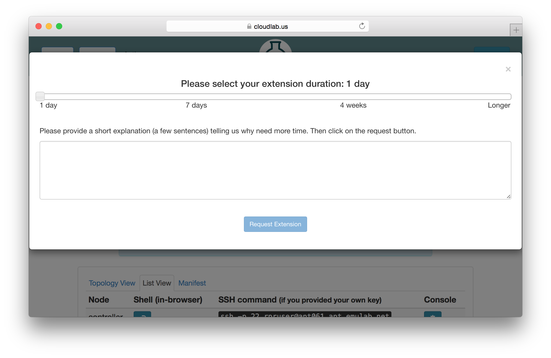
All experiments have an expiration time. By default, the expiration time is short (a few hours), but users can use the “Extend” button on the experiment page to request an extension. A request for an extension must be accompanied by a short description that explains the reason for requesting an extension, which will be reviewed by CloudLab staff. You will receive email a few hours before your experiment expires reminding you to copy your data off or request an extension.
5.2.1 Extending Experiments
If you need more time to run an experiment, you may use the “Extend” button on the experiment’s page. You will be presented with a dialog that allows you to select how much longer you need the experiment. Longer time periods require more extensive appoval processes. Short extensions are auto-approved, while longer ones require the intervention of CloudLab staff or, in the case of indefinite extensions, the steering commitee.
5.3 Projects
Users are grouped into projects. A project is, roughly speaking, a group of people working together on a common research or educational goal. This may be people in a particular research lab, a distributed set of collaborators, instructors and students in a class, etc.
A project is headed by a project leader. We require that project leaders be faculty, senior research staff, or others in an authoritative position. This is because we trust the project leader to approve other members into the project, ultimately making them responsible for the conduct of the users they approve. If CloudLab staff have questions about a project’s activities, its use of resources, etc., these questions will be directed to the project leader. Some project leaders run a lot of experiments themselves, while some choose to approve accounts for others in the project, who run most of the experiments. Either style works just fine in CloudLab.
Permissions for some operations/resources depend on the project that they belong to.
Currently, the only such permission is the ability to make a profile visible onto to the owning project. We expect to introduce more project-specific permissions features in the future.
5.4 Physical Resources
Users of CloudLab may get exclusive, low-level (root) control over physical machines. When allocated this way, no layers of virtualization or indirection get in the way of the way of performance, and users can be sure that no other users have access to the machines at the same time. This is an ideal situation for repeatable research.
Physical machines are re-imaged between users, so you can be sure that your physical machines don’t have any state left around from the previous user. You can find descriptions of the hardware in CloudLab’s clusters in the hardware chapter.
5.5 Virtual Machines
While CloudLab does have the ability to provision virtual machines (using the Xen hypervisor), we expect that the dominant use of CloudLab is that users will provision physical machines. Users (or the cloud software stacks that they run) may build their own virtual machines on these physical nodes using whatever hypervisor they wish. However, if your experiment could still benefit from use of virtual machines (e.g. to form a scalable pool of clients issuing requests to your cloud software stack), you can find more detail in the advanced topics section.
6 CloudLab for Classes
CloudLab can be a good environment for classes: it provides students with separate, isolated environments in which to do their work, and those environments can easily be brought to a known clean state so that all students get a consistent environment. Students get root access on their nodes, making CloudLab ideal for classes that require configuration or code changes to the operating system, or low-level access to the hardware. Because CloudLab is a network testbed, it is also idea for class projects that make use of multiple nodes.
There are some limitations that you should be aware of before deciding to use CloudLab for a class:
CloudLab has limited resources: in large classes, if students leave work to the last minute, or all students try to work on a deadline at the same time, they may run into problems getting the nodes they need in time.
CloudLab has a policy that resources can only be held while they are actively being used. Make sure that students are aware that individual resource allocations are not meant to last all quarter/semester: students should start experiments when they are ready to begin work, and terminate them when they are done.
You will want to make sure that students understand that storage on nodes in CloudLab is ephemeral and will be cleared out when experiments terminate. Addtionally, while CloudLab makes every effort to provide a reliable service, hardware failures, etc. can cause data loss. Students need to be sure to regularly copy off important work to avoid loss due to experiment termination or equipment failures.
Resource reservations can be useful for classes: they ensure that a certain number of resources are available for use by a project during a specified time period. It’s important to note that the resource pool is shared by all members of the project: for example, if you reserve 10 nodes, they can be used by up to 10 different experiments. Students do not need to do anything special to use these reservations: simply starting an experiment during the reservation period will automatically make use of the reservation.
If you have any questions about using CloudLab for classes, see the getting help chapter of this manual. We ask that instructors and TAs be the primary point of contact for students in requesting help with CloudLab: CloudLab has a small support staff that cannot handle a large volume of student support.
6.1 Creating Your Project on CloudLab
Students should not apply for their own projects on CloudLab: the instructor or an assistant (such as a TA) should apply for a project. Be sure to check the box indicating that the project is for a class, and include enough information in the application for us to have a look at the class, such as a link to the syllabus if available.
We ask that you create a new project for each class that you teach; eg. each quarter/semester of a course should apply for a new project on CloudLab. If course staff (instructors, TAs, etc.) already have an account on CloudLab, they can re-use their existing accounts: simply log in before applying for the new project.
Once the project has been approved, students will apply to join it as described below. Course staff can approve these accounts, without CloudLab staff having to get involved. One way to smooth the process of approving accounts for large classes is to allow TAs to approve them; when approving a new account, you may give it "manager" permissions, which allows the account to approve others. You may also give users this status via the "Members" tab of the project page at any time.
6.2 Having Students Join Your Project
When a CloudLab project is approved, the project leader will receive an email with a link to join the project. This link can be distributed to students in the course, who will use it to apply for an account. Once a student applies, the project leader will receive email with the application, and can approve or deny it. Alternately, students can join the project by following the standard CloudLab "join an existing project" instructions, and enter the name of the class’s project.
Students who apply to start their own project will have their project requests denied, and be asked to join the main project for the class.
Students who already have an account on CloudLab can join the project without making a new account; simply log in before applying to join the new project.
6.3 Project-Based Classes
Classes that are based around students working independently or in groups are an ideal use case for CloudLab; all members of the project are given logins on all experiments started under the project, which enables easy collaboration.
6.4 Assignment-Based Classes
For classes in which all students are working on the same task, it can be useful to either use an existing profile or create a new one. This way, all students will have the same environment, simplifying instructions and making debugging easier. The page for each profile has a "share" button that can be used to get a link to include with the assignment.
For large classes, we recommend considering whether virtual machines can meet students’ needs, as this reduces the resource load on CloudLab. Virtual machines should use shared mode so that they run on shared, not exclusive, hosts.
All members of a project are given shells on all experiments in the project: thus, TAs can log into nodes being used by students to help examine or debug code.
7 Resource Reservations
CloudLab supports reservations that allow you to request resources ahead of time. This can be useful for tutorials, classes, and to run larger experiments than are typically possible on a first-come, first-served basis.
Reservations in CloudLab are per-cluster and per-type. They are tied to a project: an experiment must belong to that project to use the reserved nodes (in some cases, the scope of reservations might be further restricted to experiments associated with a particular user, or a particular subgroup). For homogeneous groups of resources (such as compute nodes of the same type), reservations are not tied to specific nodes; this gives CloudLab maximum flexibility to do late-binding of nodes to experiments instantiated from reservations, which makes them minimally intrusive on other users of the testbed.
7.1 What Reservations Guarantee
Having a reservation guarantees that, at minimum, the specified quantity of nodes of the specified type will be available for use by the project during the specified time window.
Having a reservation does not automatically start an experiment at that time: it ensures that the specified number of nodes are available for use by any experiments that you (or in some cases, your fellow project members) start.
More than one experiment may use nodes from the reservation; for example, a tutorial in which 40 students each will run an experiment having a single node may be handled as a single 40-node reservation. You may also start and terminate multiple experiments in series over the course of the reservation: reserved nodes will not be returned to general use until your reservation ends.
A reservation guarantees the minimum number of nodes that will be available; you may use more so long as they are not used by other experiments or reservations.
Experiments run during a reservation do not automatically terminate at the end of the reservation; they simply become subject to the normal resource usage policies, and, for example, may become non-extendable due to other reservations that start after yours.
Important caveats include:
Nodes can take several minutes to be freed and reloaded between experiments; this means that they may take a few minutes to be available at the beginning of your reservation, and if you terminate an experiment during your reservation, they may take a few minutes to be usable for your next experiment.
The reservation system cannot account for factors outside of its control such as hardware failures; this many result in occasional failures to get the full number of nodes in exceptional circumstances.
The reservation system ensures that enough nodes of the specified type are available, but does not consider other factors such as network topology, and so cannot guarantee that all possible experiments can be started, even if they fit within the number of nodes.
7.2 How Reservations May Affect You
Reservations held by others may affect your experiments in two ways: they may prevent you from creating new experiments or may prevent you from extending existing experiments. This “admission control system” is how we ensure that nodes are available for those that have them reserved.
If there is an ongoing or upcoming reservation by another project, you may encounter an “admission control” failure when trying to create a new experiment. This means that, although there are enough nodes that are not currently allocated to a particular experiment, some or all of those nodes are required in order to fulfill a reservation. Note that the admission control system assumes that your experiment will last for the full default experiment duration when making this calcuation. For example, if the default experiment duration is 24 hours, and a large reservation will start in 10 hours, your experiment may fail to be created due to the admission control system. If the large reservation starts in 30 hours, you will be able to create the experiment, but you may not be able to extend it.
Reservations can also prevent you from extending existing experiments, if that extension would cause too few nodes to be available to satisfy a reservation. A message will appear on the experiment’s status page warning you when this situation will occur in the near future, and the reservation request dialog will limit the length of reservation that you can request. If this happens, be sure to save all of your work, as the administrators cannot grant extensions that would interfere with reservations.
7.3 Making a Reservation
To request a reservation, use the “Reserve Nodes” item from the “Experiments” menu.
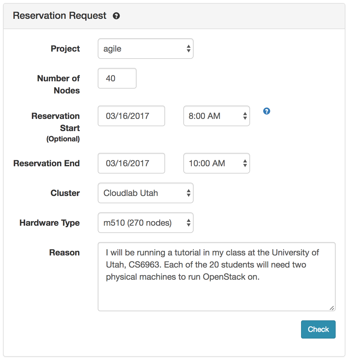
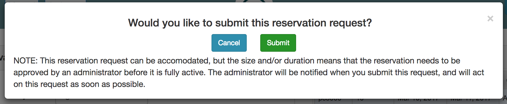
After filling out the number of and type of nodes and the time, the check button checks to see if the reservation is possible. If your request is satisfiable, you will get a dialog box that lets you submit the request.
If your request is not satisfiable, you will be given a chance to modify the request and “check” again. In this case, the time when there will not be enough nodes is shown, as will the number of nodes by which the request exceeds availalbe resources. To make your reservation fit, try asking for a different type of nodes, a smaller number, or a time further in the future.
Not all reservation requests are automatically accepted. Your request will be shown as “pending” while it is being reviewed by the CloudLab administrators. Requesting the smaller numbers of nodes, or for shorter periods of time, will maximize the chances that youre request is accepted. Be sure to include meaningful text in the “Reason” field, as administrators will use this to determine whether to grant your reservation.
You may have more than one reservation at a time; if you need resources of more than one type, or on different clusters, you can get this by requesting mutliple reservations.
7.4 Using a Reservation
To use a reservation, simply create experiments as normal. Experiments run during the duration of the reservation (even those begun before its start time) are automatically counted towards the reservation. Experiments run during reservations have expiration times as do normal experiments, so be sure to extend them if necessary.
Since reservations are associated with a project, if you belong to more than one, make sure to create the experiment under the correct project. (If the project is organised into subgroups, selecting the appropriate subgroup might also be necessary.)
Experiments are not automatically terminated at the conclusion of a reservation (though it may not be possible to extend them due to other reservations). Remember to terminate your experiments when you are done with them, as you would do normally.
If you finish your work, and still have any active experiments or related reservations, we ask that you terminate the associated experiments and delete the reservations so that the resources can be freed up for use by others.
7.5 Who Shares Access to Reservations
As mentioned above, every reservation is tied to exactly one project, and experiments belonging to other projects will be excluded from reserved resources for the duration of the reservation.
Different projects can have very different organisational models, however. One project might be run by a manager (such as a class instructor) who makes reservations on behalf of the entire project, and then individual project members start experiments each using a fraction of the reserved resources. Another project might operate informally, and its project members behave independently: those members might prefer to make private reservations for their own use (excluding their fellow project members from intentionally or unintentionally consuming the reserved resources with experiments of their own).
(Some projects are organised hierarchically, and make use of subgroups within the project; reservations can also be handled by subgroup, if applicable.)
CloudLab offers three reservation sharing options a project may choose from:
By user |
| An experiment will be able to access reserved resources only if the experiment and reservation are in the same project, and the experiment was started by the same user who requested the reservation. |
By project |
| An experiment will be able to access reserved resources only if the experiment and reservation are in the same project. |
By subgroup |
| An experiment will be able to access reserved resources only if the experiment and reservation are in the same project, and the experiment and the reservation specify the same subgroup. |
A project leader can request the reservation sharing semantics suitable for their project by contacting support@cloudlab.us.
Please note that the sharing semantics of reservations must be chosen (by the project leader) for the project as a whole. It is not possible to request a custom scope for individual reservations.
8 Describing a profile with python and geni-lib
See the geni-lib manual
geni-lib is a tool that allows users to generate RSpec files from Python code. CloudLab offers the ability to use geni-lib scripts as the definition of a profile, rather then the more primitive RSpec format. When you supply a geni-lib script on the Create Profile page, your script is uploaded to the server so that it can be executed in the geni-lib environment. This allows the script to be verified for correctness, and also produces the equivalent RSpec representation that you can view if you so desire.
When you provide a geni-lib script, you will see a slightly different set of buttons on the Create Profile page; next to the “Source” button there is an “XML” button that will pop up the RSpec XML for you to look at. The XML is read-only; if you want to change the profile, you will need to change the python source code that is displayed when you click on the “Source” button. Each time you change the python source code, the script is uploaded to the server and processed. Be sure to save your changes if you are updating an existing profile.
The following examples demonstrate basic geni-lib usage. More information about geni-lib and additional examples, can be found in the geni-lib repository. Its full documentation is online as part of this manual.
8.1 A single XEN VM node
"""An example of constructing a profile with a single Xen VM. Instructions: Wait for the profile instance to start, and then log in to the VM via the ssh port specified below. (Note that in this case, you will need to access the VM through a high port on the physical host, since we have not requested a public IP address for the VM itself.) """ # Import the Portal object. import geni.portal as portal import geni.rspec.pg as rspec # Create a Request object to start building the RSpec. request = portal.context.makeRequestRSpec() # Add a XenVM (named "node") to the request node = request.XenVM("node") # Write the request in RSpec format portal.context.printRequestRSpec() Open this profile on CloudLab"""An example of constructing a profile with a single Xen VM. Instructions: Wait for the profile instance to start, and then log in to the VM via the ssh port specified below. (Note that in this case, you will need to access the VM through a high port on the physical host, since we have not requested a public IP address for the VM itself.) """ # Import the Portal object. import geni.portal as portal import geni.rspec.pg as rspec # Create a Request object to start building the RSpec. request = portal.context.makeRequestRSpec() # Add a XenVM (named "node") to the request node = request.XenVM("node") # Write the request in RSpec format portal.context.printRequestRSpec()
This example demonstrates the two most important objects: the portal context (accessed through the portal.context object in the geni.portal module), and the request RSpec created by calling makeRequestRSpec() on it. These fundamental objects are central to essentially all CloudLab geni-lib profiles.
Another way to create a Request RSpec object is to call its constructuor, geni.rspec.pg.Request directly. We ask the Context to create it for us so it it is "bound" to the context and does not need to be explicitly passed to other functions on the context
Once the request object has been created, resources may be added to it by calling methods on it like RawPC() or rspec.pg.LAN. In this example, just a single node (created with the XenVM() constructor, asking for a single VM identified by the name "node") is requested.
Most functions called on Request objects are not directly members of that class. Rather, they are loaded as "extensions" by modules such as geni.rspec.emulab.
The final action the geni-lib script performs is to generate the XML representation of the request RSpec, with the printRequestRSpec() call on the last line. This has the effect of communicating the description of all the resources requested by the profile back to CloudLab.
You will also notice that the profile begins with a string literal (to be precise, it is a Python docstring). The initial text will also be used as the profile description; the text following the Instructions: line will be used as the corresponding instructions. This documentation is so important that adding the description to the profile is mandatory. (Using a docstring like this is not the only way to produce the description and instructions, although it is the most convenient.)
This simple example has now demonstrated all the important elements of a geni-lib profile. The portal context and request RSpec objects, the final printRequestRSpec() call, and the docstring description and instructions are “boilerplate” constructions, and you will probably include similar or identical versions of them in every geni-lib profile you create unless you are doing something quite unusual.
8.2 A single physical host
"""An example of constructing a profile with a single raw PC. Instructions: Wait for the profile instance to start, and then log in to the host via the ssh port specified below. """ import geni.portal as portal import geni.rspec.pg as rspec # Create a Request object to start building the RSpec. request = portal.context.makeRequestRSpec() # Create a raw PC node = request.RawPC("node") # Print the RSpec to the enclosing page. portal.context.printRequestRSpec() Open this profile on CloudLab"""An example of constructing a profile with a single raw PC. Instructions: Wait for the profile instance to start, and then log in to the host via the ssh port specified below. """ import geni.portal as portal import geni.rspec.pg as rspec # Create a Request object to start building the RSpec. request = portal.context.makeRequestRSpec() # Create a raw PC node = request.RawPC("node") # Print the RSpec to the enclosing page. portal.context.printRequestRSpec()
As mentioned above, most of these simple examples consist of boilerplate geni-lib fragments, and indeed the portal context and request RSpec operations are unchanged from the previous script. The big difference, though (other than the updated documentation) is that in this case the RawPC() method is invoked on the Request object instead of XenVM(). As you might expect, the new profile will request a physical host instead of a virtual one. (A side effect of using a real machine is that it automatically comes with a unique public IP address, where the VM used in the earlier example did not. Profiles can request public IP addresses for VMs too, though it does not happen by default.)
8.3 Two XenVM nodes with a link between them
"""An example of constructing a profile with two VMs connected by a LAN. Instructions: Wait for the profile instance to start, and then log in to either VM via the ssh ports specified below. """ import geni.portal as portal import geni.rspec.pg as rspec request = portal.context.makeRequestRSpec() # Create two XenVM nodes. node1 = request.XenVM("node1") node2 = request.XenVM("node2") # Create a link between them link1 = request.Link(members = [node1,node2]) portal.context.printRequestRSpec() Open this profile on CloudLab"""An example of constructing a profile with two VMs connected by a LAN. Instructions: Wait for the profile instance to start, and then log in to either VM via the ssh ports specified below. """ import geni.portal as portal import geni.rspec.pg as rspec request = portal.context.makeRequestRSpec() # Create two XenVM nodes. node1 = request.XenVM("node1") node2 = request.XenVM("node2") # Create a link between them link1 = request.Link(members = [node1,node2]) portal.context.printRequestRSpec()
This example demonstrates two important geni-lib concepts: first, adding more than a single node to the request (which is a relatively straightforward matter of calling more than one node object constructor, being careful to use a different name each time). It also shows how to add links between nodes. It is possible to construct links and LANs in a more complicated manner (such as explicitly creating Interface objects to control interfaces), but the simplest case is to supply the member nodes at the time the link is created.
8.4 Two ARM64 servers in a LAN
"""An example of constructing a profile with two ARM64 nodes connected by a LAN. Instructions: Wait for the profile instance to start, and then log in to either host via the ssh ports specified below. """ import geni.portal as portal import geni.rspec.pg as rspec request = portal.context.makeRequestRSpec() # Create two raw "PC" nodes node1 = request.RawPC("node1") node2 = request.RawPC("node2") # Set each of the two to specifically request "m400" nodes, which in CloudLab, are ARM node1.hardware_type = "m400" node2.hardware_type = "m400" # Create a link between them link1 = request.Link(members = [node1, node2]) portal.context.printRequestRSpec() Open this profile on CloudLab"""An example of constructing a profile with two ARM64 nodes connected by a LAN. Instructions: Wait for the profile instance to start, and then log in to either host via the ssh ports specified below. """ import geni.portal as portal import geni.rspec.pg as rspec request = portal.context.makeRequestRSpec() # Create two raw "PC" nodes node1 = request.RawPC("node1") node2 = request.RawPC("node2") # Set each of the two to specifically request "m400" nodes, which in CloudLab, are ARM node1.hardware_type = "m400" node2.hardware_type = "m400" # Create a link between them link1 = request.Link(members = [node1, node2]) portal.context.printRequestRSpec()
We now come to demonstrate requesting particular properties of nodes—
8.5 A VM with a custom size
"""An example of constructing a profile with a single Xen VM. Instructions: Wait for the profile instance to start, and then log in to the VM via the ssh port specified below. (Note that in this case, you will need to access the VM through a high port on the physical host, since we have not requested a public IP address for the VM itself.) """ import geni.portal as portal import geni.rspec.pg as rspec # Create a Request object to start building the RSpec. request = portal.context.makeRequestRSpec() # Create a XenVM node = request.XenVM("node") # Ask for two cores node.cores = 2 # Ask for 2GB of ram node.ram = 2048 # Add an extra 8GB of space on the primary disk. # NOTE: Use fdisk, the extra space is in the 4th DOS partition, # you will need to create a filesystem and mount it. node.disk = 8 # Alternate method; request an ephemeral blockstore mounted at /mydata. # NOTE: Comment out the above line (node.disk) if you do it this way. #bs = node.Blockstore("bs", "/mydata") #bs.size = "8GB" #bs.placement = "nonsysvol" # Print the RSpec to the enclosing page. portal.context.printRequestRSpec() Open this profile on CloudLab"""An example of constructing a profile with a single Xen VM. Instructions: Wait for the profile instance to start, and then log in to the VM via the ssh port specified below. (Note that in this case, you will need to access the VM through a high port on the physical host, since we have not requested a public IP address for the VM itself.) """ import geni.portal as portal import geni.rspec.pg as rspec # Create a Request object to start building the RSpec. request = portal.context.makeRequestRSpec() # Create a XenVM node = request.XenVM("node") # Ask for two cores node.cores = 2 # Ask for 2GB of ram node.ram = 2048 # Add an extra 8GB of space on the primary disk. # NOTE: Use fdisk, the extra space is in the 4th DOS partition, # you will need to create a filesystem and mount it. node.disk = 8 # Alternate method; request an ephemeral blockstore mounted at /mydata. # NOTE: Comment out the above line (node.disk) if you do it this way. #bs = node.Blockstore("bs", "/mydata") #bs.size = "8GB" #bs.placement = "nonsysvol" # Print the RSpec to the enclosing page. portal.context.printRequestRSpec()
The earlier examples requesting VMs used the default number of cores, quantity of RAM, and disk size. It’s also possible to customize these value, as this example does by setting the cores, ram, and disk properties of the XenVM class (which is a subclass of rspec.pg.Node.)
8.6 Set a specific IP address on each node
"""An example of constructing a profile with node IP addresses specified manually. Instructions: Wait for the profile instance to start, and then log in to either VM via the ssh ports specified below. (Note that even though the EXPERIMENTAL data plane interfaces will use the addresses given in the profile, you will still connect over the control plane interfaces using addresses given by the testbed. The data plane addresses are for intra-experiment communication only.) """ import geni.portal as portal import geni.rspec.pg as rspec request = portal.context.makeRequestRSpec() node1 = request.XenVM("node1") iface1 = node1.addInterface("if1") # Specify the component id and the IPv4 address iface1.component_id = "eth1" iface1.addAddress(rspec.IPv4Address("192.168.1.1", "255.255.255.0")) node2 = request.XenVM("node2") iface2 = node2.addInterface("if2") # Specify the component id and the IPv4 address iface2.component_id = "eth2" iface2.addAddress(rspec.IPv4Address("192.168.1.2", "255.255.255.0")) link = request.LAN("lan") link.addInterface(iface1) link.addInterface(iface2) portal.context.printRequestRSpec() Open this profile on CloudLab"""An example of constructing a profile with node IP addresses specified manually. Instructions: Wait for the profile instance to start, and then log in to either VM via the ssh ports specified below. (Note that even though the EXPERIMENTAL data plane interfaces will use the addresses given in the profile, you will still connect over the control plane interfaces using addresses given by the testbed. The data plane addresses are for intra-experiment communication only.) """ import geni.portal as portal import geni.rspec.pg as rspec request = portal.context.makeRequestRSpec() node1 = request.XenVM("node1") iface1 = node1.addInterface("if1") # Specify the component id and the IPv4 address iface1.component_id = "eth1" iface1.addAddress(rspec.IPv4Address("192.168.1.1", "255.255.255.0")) node2 = request.XenVM("node2") iface2 = node2.addInterface("if2") # Specify the component id and the IPv4 address iface2.component_id = "eth2" iface2.addAddress(rspec.IPv4Address("192.168.1.2", "255.255.255.0")) link = request.LAN("lan") link.addInterface(iface1) link.addInterface(iface2) portal.context.printRequestRSpec()
This code sample assigns specific IP addresses to interfaces on the nodes it requests.
Some of the available qualifiers on requested nodes are specified by manipulating attributes within the node (or interface) object directly. The hardware_type in the previous example is one such case, as is the component_id here. (Note that the component_id in this example is applied to an interface, although it is also possible to specify component_ids on nodes, too, to request a particular physical host.)
Other modifications to requests require dedicated methods. For instance, see the addAddress() calls made on each of the two interfaces above. In each case, an IPv4Address object is obtained from the appropriate constructor (the parameters are the address and the netmask, respectively), and then added to the corresponding interface.
8.7 Specify an operating system and set install and execute scripts
"""An example of constructing a profile with install and execute services. Instructions: Wait for the profile instance to start, then click on the node in the topology and choose the `shell` menu item. The install and execute services are handled automatically during profile instantiation, with no manual intervention required. """ # Import the Portal object. import geni.portal as portal # Import the ProtoGENI library. import geni.rspec.pg as rspec # Create a Request object to start building the RSpec. request = portal.context.makeRequestRSpec() # Add a raw PC to the request. node = request.RawPC("node") # Request that a specific image be installed on this node node.disk_image = "urn:publicid:IDN+emulab.net+image+emulab-ops//UBUNTU20-64-STD"; # Install and execute scripts on the node. THIS TAR FILE DOES NOT ACTUALLY EXIST! node.addService(rspec.Install(url="http://example.org/sample.tar.gz", path="/local")) node.addService(rspec.Execute(shell="bash", command="/local/example.sh")) portal.context.printRequestRSpec()Open this profile on CloudLab"""An example of constructing a profile with install and execute services. Instructions: Wait for the profile instance to start, then click on the node in the topology and choose the `shell` menu item. The install and execute services are handled automatically during profile instantiation, with no manual intervention required. """ # Import the Portal object. import geni.portal as portal # Import the ProtoGENI library. import geni.rspec.pg as rspec # Create a Request object to start building the RSpec. request = portal.context.makeRequestRSpec() # Add a raw PC to the request. node = request.RawPC("node") # Request that a specific image be installed on this node node.disk_image = "urn:publicid:IDN+emulab.net+image+emulab-ops//UBUNTU20-64-STD"; # Install and execute scripts on the node. THIS TAR FILE DOES NOT ACTUALLY EXIST! node.addService(rspec.Install(url="http://example.org/sample.tar.gz", path="/local")) node.addService(rspec.Execute(shell="bash", command="/local/example.sh")) portal.context.printRequestRSpec()
This example demonstrates how to request services for a node, where CloudLab will automate some task as part of the profile instance setup procedure. In this case, two services are described (an install and an execute). This is a very common pair of services to request together: the Install object describes a service which retrieves a tarball from the location given in the url parameter, and installs it into the local filesystem as specified by path. (The installation occurs during node setup, upon the first boot after the disk image has been loaded.) The second service, described by the Execute object, invokes a shell process to run the given command. In this example (as is common), the command refers directly to a file saved by the immediately preceding Install service. This behaviour works, because CloudLab guarantees that all Install services complete before any Execute services are started. The command executes every time the node boots, so you can use it start daemons, etc. that are necessary for your experiment.
8.8 Profiles with user-specified parameters
"""An example of using parameters to construct a profile with a variable number of nodes. Instructions: Wait for the profile instance to start, and then log in to one or more of the VMs via the ssh port(s) specified below. """ # Import the Portal object. import geni.portal as portal # Import the ProtoGENI library. import geni.rspec.pg as rspec # Describe the parameter(s) this profile script can accept. portal.context.defineParameter( "n", "Number of VMs", portal.ParameterType.INTEGER, 1 ) # Retrieve the values the user specifies during instantiation. params = portal.context.bindParameters() # Create a Request object to start building the RSpec. request = portal.context.makeRequestRSpec() # Check parameter validity. if params.n < 1 or params.n > 8: portal.context.reportError( portal.ParameterError( "You must choose at least 1 and no more than 8 VMs.", ["n"] ) ) # Abort execution if there are any errors, and report them. portal.context.verifyParameters() for i in range( params.n ): # Create a XenVM and add it to the RSpec. node = request.XenVM( "node" + str( i ) ) # Print the RSpec to the enclosing page. portal.context.printRequestRSpec() Open this profile on CloudLab"""An example of using parameters to construct a profile with a variable number of nodes. Instructions: Wait for the profile instance to start, and then log in to one or more of the VMs via the ssh port(s) specified below. """ # Import the Portal object. import geni.portal as portal # Import the ProtoGENI library. import geni.rspec.pg as rspec # Describe the parameter(s) this profile script can accept. portal.context.defineParameter( "n", "Number of VMs", portal.ParameterType.INTEGER, 1 ) # Retrieve the values the user specifies during instantiation. params = portal.context.bindParameters() # Create a Request object to start building the RSpec. request = portal.context.makeRequestRSpec() # Check parameter validity. if params.n < 1 or params.n > 8: portal.context.reportError( portal.ParameterError( "You must choose at least 1 and no more than 8 VMs.", ["n"] ) ) # Abort execution if there are any errors, and report them. portal.context.verifyParameters() for i in range( params.n ): # Create a XenVM and add it to the RSpec. node = request.XenVM( "node" + str( i ) ) # Print the RSpec to the enclosing page. portal.context.printRequestRSpec()
Until now, all of the geni-lib scripts have described profiles which could also have been generated with the Jacks GUI, or even by writing a raw XML RSpec directly. However, geni-lib profiles offer an important feature unavailable by the other methods: the ability to describe not a static request, but a request “template” which is dynamically constructed based on a user’s choices at the time the profile is instantiated. The mechanism for constructing such profiles relies on profile parameters; the geni-lib script describes the set of parameters it will accept, and then retrieves the corresponding values at instantiation time and is free to respond by constructing arbitrarily different resource requests based on that input.
The profile above accepts exactly one parameter—
| Simple integer | |
| Arbitrary (uninterpreted) string | |
| True or False | |
| URN to a disk image | |
| URN of a GENI Aggregate Manager | |
| String specifying a type of node | |
| Floating-point number specifying bandwidth in kbps | |
| Floating-point number specifying delay in ms | |
| Integer used for memory or disk size (e.g., MB, GB, etc.) |
The last field is the default value of the parameter, and is required: not only must the field itself contain a valid value, but the set of all parameters must be valid when each of them assumes the default value. (This is partly so that the portal can construct a default topology for the profile without any manual intervention, and partly so that unprivileged users, who may lack permission to supply their own values, might still be able to instantiate the profile.)
After all parameters have been defined, the profile script may retrieve the runtime values with the bindParameters() method. This will return a Python class instance with one attribute for each parameter (with the name supplied during the appropriate defineParameter() call). In the example, the instance was assigned to params, and therefore the only parameter (which was called "n") is accessible as params.n.
Of course, it may be possible for the user to specify nonsensical values for a parameter, or perhaps give a set of parameters whose combination is invalid. A profile should detect error cases like these, and respond by constructing a portal.ParameterError object, which can be passed to the portal context’s reportError() method to abort generation of the RSpec. By default, reportError() does not abort the script immediately unless you pass it a specific argument; see its documentation for more detail. If you prefer to allow all errors and warnings to be generated, and to only abort the script at that point, and prior to creating RSpec resources, you can manually call verifyParameters() after completing parameter value checks. verifyParameters() is also automatically invoked prior to printing the request RSpec, so if your script can function despite malformed parameter values, you do not need to manually call verifyParameters().
8.9 Add storage to a node
Adding extra temporary diskspace to a node using a node-local dataset,
Creating a reusable dataset from local disk space using an image-backed dataset,
Adding network-attached storage to a node using a remote dataset,
Safely read-write sharing a remote dataset on multiple nodes via NFS,
Using read-write clones of a remote dataset on multiple nodes
8.10 Debugging geni-lib profile scripts
It is not necessary to instantiate the profile via the portal web interface
to test it. Properly written profile scripts should work perfectly well
independent of the normal portal—
python geni-lib-parameters.py
will produce an RSpec containing three nodes (the default value for n). It is also possible to override the defaults on the command line by giving the parameter name as an option, followed by the desired value:
python geni-lib-parameters.py –n 4
The option –help will list the available parameters and their descriptions.
9 Virtual Machines
A CloudLab virtual node is a virtual machine running on top of a regular operating system. CloudLab virtual nodes are based on the Xen hypervisor, which allows groups of processes to be isolated from each other while running on the same physical machine. CloudLab virtual nodes provide isolation of the filesystem, process, network, and account namespaces. Thus, each virtual node has its own private filesystem, process hierarchy, network interfaces and IP addresses, and set of users and groups. This level of virtualization allows unmodified applications to run as though they were on a real machine. Virtual network interfaces support an arbitrary number of virtual network links. These links may be individually shaped according to user-specified link parameters, and may be multiplexed over physical links or used to connect to virtual nodes within a single physical node.
There are a few specific differences between virtual and physical nodes. First, CloudLab physical nodes have a routable, public IPv4 address allowing direct remote access (unless the CloudLab installation has been configured to use unroutable control network IP addresses, which is very rare). However, virtual nodes are assigned control network IP addresses on a private network (typically the 172.16/12 subnet) and are remotely accessible over ssh via DNAT (destination network-address translation) to the physical host’s public control network IP address, to a high-numbered port. Depending on local configuration, it may be possible to request routable IP addresses for specific virtual nodes to enable direct remote access. Note that virtual nodes are always able to access the public Internet via SNAT (source network-address translation; nearly identical to masquerading).
Second, virtual nodes and their virtual network interfaces are connected by virtual links built atop physical links and physical interfaces. The virtualization of a physical device/link decreases the fidelity of the network emulation. Moreover, several virtual links may share the same physical links via multiplexing. Individual links are isolated at layer 2, but they are not isolated in terms of performance. If you request a specific bandwidth for a given set of links, our resource mapper will ensure that if multiple virtual links are mapped to a single physical link, the sum of the bandwidths of the virtual links will not exceed the capacity of the physical link (unless you also specify that this constraint can be ignored by setting the best_effort link parameter to True). For example, no more than ten 1Gbps virtual links can be mapped to a 10Gbps physical link.
Finally, when you allocate virtual nodes, you can specify the amount of CPU and RAM (and, for Xen VMs, virtual disk space) each node will be allocated. CloudLab’s resource assigner will not oversubscribe these quantities.
9.1 Xen VMs
These examples show the basics of allocating Xen VMs: a single Xen VM node, two Xen VMs in a LAN, a Xen VM with custom disk size. In the sections below, we discuss advanced Xen VM allocation features.
9.1.1 Controlling CPU and Memory
You can control the number of cores and the amount of memory allocated to each VM by setting the cores and ram instance variables of a XenVM object, as shown in the following example:
"""An example of constructing a profile with a single Xen VM. Instructions: Wait for the profile instance to start, and then log in to the VM via the ssh port specified below. (Note that in this case, you will need to access the VM through a high port on the physical host, since we have not requested a public IP address for the VM itself.) """ import geni.portal as portal import geni.rspec.pg as rspec # Create a Request object to start building the RSpec. request = portal.context.makeRequestRSpec() # Create a XenVM node = request.XenVM("node") # Request a specific number of VCPUs. node.cores = 4 # Request a specific amount of memory (in MB). node.ram = 4096 # Print the RSpec to the enclosing page. portal.context.printRequestRSpec() """An example of constructing a profile with a single Xen VM. Instructions: Wait for the profile instance to start, and then log in to the VM via the ssh port specified below. (Note that in this case, you will need to access the VM through a high port on the physical host, since we have not requested a public IP address for the VM itself.) """ import geni.portal as portal import geni.rspec.pg as rspec # Create a Request object to start building the RSpec. request = portal.context.makeRequestRSpec() # Create a XenVM node = request.XenVM("node") # Request a specific number of VCPUs. node.cores = 4 # Request a specific amount of memory (in MB). node.ram = 4096 # Print the RSpec to the enclosing page. portal.context.printRequestRSpec()
9.1.2 Controlling Disk Space
Each Xen VM is given enough disk space to hold the requested image. Most CloudLab images are built with a 16 GB root partition, typically with about 25% of the disk space used by the operating system. If the remaining space is not enough for your needs, you can request additional disk space by setting a XEN_EXTRAFS node attribute, as shown in the following example.
"""An example of constructing a profile with a single Xen VM with extra fs space. Instructions: Wait for the profile instance to start, and then log in to the VM via the ssh port specified below. (Note that in this case, you will need to access the VM through a high port on the physical host, since we have not requested a public IP address for the VM itself.) """ import geni.portal as portal import geni.rspec.pg as rspec # Import Emulab-specific extensions so we can set node attributes. import geni.rspec.emulab as emulab # Create a Request object to start building the RSpec. request = portal.context.makeRequestRSpec() # Create a XenVM node = request.XenVM("node") # Set the XEN_EXTRAFS to request 8GB of extra space in the 4th partition. node.Attribute('XEN_EXTRAFS','8') # Print the RSpec to the enclosing page. portal.context.printRequestRSpec() """An example of constructing a profile with a single Xen VM with extra fs space. Instructions: Wait for the profile instance to start, and then log in to the VM via the ssh port specified below. (Note that in this case, you will need to access the VM through a high port on the physical host, since we have not requested a public IP address for the VM itself.) """ import geni.portal as portal import geni.rspec.pg as rspec # Import Emulab-specific extensions so we can set node attributes. import geni.rspec.emulab as emulab # Create a Request object to start building the RSpec. request = portal.context.makeRequestRSpec() # Create a XenVM node = request.XenVM("node") # Set the XEN_EXTRAFS to request 8GB of extra space in the 4th partition. node.Attribute('XEN_EXTRAFS','8') # Print the RSpec to the enclosing page. portal.context.printRequestRSpec()
This attribute’s unit is in GB. As with CloudLab physical nodes, the extra disk space will appear in the fourth partition of your VM’s disk. You can turn this extra space into a usable file system by logging into your VM and doing:
mynode> sudo mkdir /dirname mynode> sudo /usr/local/etc/emulab/mkextrafs.pl /dirname
where dirname is the directory you want your newly-formatted file system to be mounted.
"""An example of constructing a profile with a single Xen VM. Instructions: Wait for the profile instance to start, and then log in to the VM via the ssh port specified below. (Note that in this case, you will need to access the VM through a high port on the physical host, since we have not requested a public IP address for the VM itself.) """ import geni.portal as portal import geni.rspec.pg as rspec # Create a Request object to start building the RSpec. request = portal.context.makeRequestRSpec() # Create a XenVM node = request.XenVM("node") # Request a specific number of VCPUs. node.cores = 4 # Request a specific amount of memory (in MB). node.ram = 4096 # Print the RSpec to the enclosing page. portal.context.printRequestRSpec() """An example of constructing a profile with a single Xen VM. Instructions: Wait for the profile instance to start, and then log in to the VM via the ssh port specified below. (Note that in this case, you will need to access the VM through a high port on the physical host, since we have not requested a public IP address for the VM itself.) """ import geni.portal as portal import geni.rspec.pg as rspec # Create a Request object to start building the RSpec. request = portal.context.makeRequestRSpec() # Create a XenVM node = request.XenVM("node") # Request a specific number of VCPUs. node.cores = 4 # Request a specific amount of memory (in MB). node.ram = 4096 # Print the RSpec to the enclosing page. portal.context.printRequestRSpec()
9.1.3 Setting HVM Mode
By default, all Xen VMs are paravirtualized. If you need hardware virtualization instead, you must set a XEN_FORCE_HVM node attribute, as shown in this example:
"""An example of constructing a profile with a single Xen VM in HVM mode. Instructions: Wait for the profile instance to start, and then log in to the VM via the ssh port specified below. (Note that in this case, you will need to access the VM through a high port on the physical host, since we have not requested a public IP address for the VM itself.) """ import geni.portal as portal import geni.rspec.pg as rspec # Import Emulab-specific extensions so we can set node attributes. import geni.rspec.emulab as emulab # Create a Request object to start building the RSpec. request = portal.context.makeRequestRSpec() # Create a XenVM node = request.XenVM("node") # Set the XEN_FORCE_HVM custom node attribute to 1 to enable HVM mode: node.Attribute('XEN_FORCE_HVM','1') # Print the RSpec to the enclosing page. portal.context.printRequestRSpec() """An example of constructing a profile with a single Xen VM in HVM mode. Instructions: Wait for the profile instance to start, and then log in to the VM via the ssh port specified below. (Note that in this case, you will need to access the VM through a high port on the physical host, since we have not requested a public IP address for the VM itself.) """ import geni.portal as portal import geni.rspec.pg as rspec # Import Emulab-specific extensions so we can set node attributes. import geni.rspec.emulab as emulab # Create a Request object to start building the RSpec. request = portal.context.makeRequestRSpec() # Create a XenVM node = request.XenVM("node") # Set the XEN_FORCE_HVM custom node attribute to 1 to enable HVM mode: node.Attribute('XEN_FORCE_HVM','1') # Print the RSpec to the enclosing page. portal.context.printRequestRSpec()
You can set this attribute only for dedicated-mode VMs. Shared VMs are available only in paravirtualized mode.
9.1.4 Dedicated and Shared VMs
In CloudLab, Xen VMs can be created in dedicated or shared mode. In dedicated mode, VMs run on physical nodes that are reserved to a particular experiment, and you have root-level access to the underlying physical machine. In shared mode, VMs run on physical machines that host VMs from potentially many experiments, and users do not have access to the underlying physical machine.
To request that a VM run in dedicated mode, set its exclusive attribute to True; for example node.exclusive = True. To run it in shared mode, set this value to False.
10 Storage Mechanisms
10.1 Overview of Storage Mechanisms
CloudLab offers a convenient way to specify storage resources in a profile. A blockstore, more commonly known as a dataset, is an abstraction of a block-addressable storage container of a specified size. Think of a dataset as a virtual disk that only your experiments can access. The most common way to use a dataset’s capacity is to make a filesystem on it, though that is up to the user.
A dataset may either be local, allocated on a node disk and directly accessed by the OS, or remote, located on a shared storage server and accessible via the experiment network fabric.
Datasets may also be either ephemeral, where the content lasts only as long as its referencing experiment, or persistent, where the lifetime is independent of an experiment and can thus be used across multiple successive experiments. Note that local datasets are always ephemeral, since node disks are re-imaged after every experiment use. (There is a pseudo-dataset type, the image-backed dataset, that can be used to explicitly capture the contents of a local dataset in a reusable way). Remote datasets can be ephemeral or persistent.
Persistent datasets may be either short-term or long-term. This is a policy distinction and not a technical one. The former is intended to allow fixed-duration (e.g., one week) access to larger datasets with fewer administrative hurdles. The latter is intended for longer term (e.g., months to years) ongoing access to size-limited datasets. Long-term datasets remain alive as long as they are being regularly used, but their creation is subject to per-project quotas for total size and might require interaction with CloudLab staff.
Persistent datasets may also be cloned, giving individual nodes their own mutable copy of a dataset. Currently, these clones are ephemeral, with per-node changes lost at experiment termination. This limits their utility. In the future, we plan to allow clones to be promoted to new persistent datasets, and allowed to replace the dataset they are cloning.
Datasets are not the only form of storage available to users. There is a legacy shared NFS filesystem that allows convenient but limited concurrent sharing between nodes within and across experiments.
All local storage is ephemeral. The contents of node disks will be lost when an experiment is terminated. You are responsible for saving data from local disks.
Most of these storage mechanisms are intra-cluster only. For example, a persistent dataset at Utah cannot be directly used by an experiment running on Clemson nodes. A new dataset would have to be created at Clemson, and the content explicitly copied over by the user from the Utah dataset. Likewise, the shared NFS filesystem at one cluster is independent of the shared filesystem at another cluster. Inter-cluster sharing mechanisms, e.g., scp or rsync, must be provided by the user at this time. The one exception is the Image-backed Dataset described below, which can be moved between clusters.
All of these storage mechanisms are subject to failure. CloudLab is not a storage provider. It is ultimately up to the users to make sure that important data artifacts are preserved. Node disks in particular are prone to failure; we do not configure them in any redundant way. Infrastructure services such as the iSCSI storage servers and the NFS servers have reasonable protection against hardware failures (e.g., RAID or ZFS), but most clusters do not have off-site backup of user data. If your data is important, back it up!
The following sections more concretely describe the storage resources and workflows available to CloudLab users.
10.2 Node-Local Storage
All nodes in CloudLab have at least 100GB of local storage, in the form of one or more SSDs (SATA or NVMe), spinning disks, or both. See the Hardware section for details of the local storage available on specific node types at each cluster.
By default, all current CloudLab-provided OS images have a 64GB system (root) partition (partition 3) on the boot disk (old format images before May 2023 have only a 16GB system partition). The OS installs typically take up 1-3GBs of this space, leaving 50+GB of conveniently available storage (e.g., in /tmp). While this space is sufficient for many uses, there are times when more is desired.
10.2.1 Specifying Storage in a Profile – Local Datasets
If you know you will need additional storage before you create an experiment, then you can specify the storage needs in your profile by configuring one or more local datasets. See the Local Dataset example below. These datasets are automatically created by the CloudLab node configuration scripts at experiment instantiation. If you specify a mountpoint, the system will automatically create a filesystem in the dataset on first boot, and mount it on every boot.
Local datasets are implemented on Linux using LVM. When one or more datasets are required on a Linux node, the available storage on all drives is combined into an LVM volume group and individual datasets are allocated (striped across all involved disks) as logical volumes from that.
At this time, there is no way to specify redundancy on a local dataset. The LVM volume group and its corresponding logical volumes are effectively RAID0, and thus your experiment is susceptible to data loss due to a single disk failure. This is likely only a concern for long-lived (weeks or months) experiments.
10.2.2 Allocating Storage in a Running Experiment
If you are in a situation where an existing experiment needs more space (i.e., you did not specify a dataset in the profile), we provide a script that can be run to quickly create a new filesystem using the remaining space on the system (boot) disk:
sudo /usr/local/etc/emulab/mkextrafs.pl /mydata
This will provide you with anywhere from 90GB to 1TB, depending on the node type you are on.
It is also possible to use Linux tools to create your own partitions, filesystems, LVM, ZFS, RAID, or other storage configurations. You can also resize the OS partition on the boot disk using the setup-grow-rootfs script after setting the RESIZEROOT environment variable to specify the desired new size–either an explicit size (in GB) or zero to indicate "the rest of the available space". For example:
sudo RESIZEROOT=0 ./setup-grow-rootfs.sh
Note that manual creation of extra partitions or resizing the root partition are discouraged since the resulting configurations will only last until the experiment ends. These techniques may also create a disk configuration that cannot be persisted because the CloudLab imaging tools may not work with the resulting partitioning due to size or layout constraints.
10.2.3 Persisting Local Data
Since most CloudLab nodes are directly accessible from the Internet, you can use your favorite tools (e.g., tar/scp or rsync) to offload your data from a node to your home before the experiment, terminates. You can copy data from local disks to the shared NFS filesystem, but this practice is strongly discouraged.
You can also make your data part of a custom OS image. By placing it in a directory like /data, it will be included in any snapshot you make. Do not put it in your home directory on the node, or transient locations like /tmp or /var/tmp as those are not captured in snapshots. This practice of “baking” data into an OS image is generally not a good idea as it ties the data to a specific OS and can result in very large images which might put you over disk quota.
CloudLab does provide one way to persist local disk data in a format that can be loaded on future experiment nodes independent of the OS image used and can be exported to other clusters. These Image-backed Datasets are described next.
10.3 Image-backed Datasets
An image-backed dataset is a snapshot of a local dataset created using a CloudLab Disk Image. Since disk images can be used across clusters, an image-backed dataset is a convenient way of both persisting data from a node and enabling it to be used in different experiments on different clusters.
An image-backed dataset can be updated from any node on which it is installed by taking a snapshot as you would an OS image. However, image-backed datasets are not versioned, there is always only one version of the dataset across all clusters. Note also that creating a new version of the dataset does not affect other currently installed copies of the dataset on other nodes. While the portal will not allow simultaneous snapshots of the same dataset, it is ultimately up to the user to ensure consistency across uses of the dataset.
An image-backed dataset can be protected as readable (install-able) by just members of your project or by anyone. Independently, they can be protected as writable (update-able) either by just yourself or by members of your project.
Examples of creation, use and updating of an image-backed dataset are shown in the Storage Examples section.
Note that the size of image-backed datasets is limited by individual clusters. Typically, this limit is around 20GB of compressed data per image, so these datasets are not well suited to very large datasets.
Note also that image-backed datasets, like all CloudLab images, are in the custom frisbee format and cannot be easily examined or used outside of CloudLab. See the Disk Images section for an overview of CloudLab images.
10.4 Remote Datasets
Remote datasets are network accessible storage volumes. Specifically, they are hosted on per-cluster, infrastructure-provided storage servers and exposed to experiment nodes via the iSCSI protocol on the experiment network fabric. Most, but not all, cluster in CloudLab have at least one storage server. See the Hardware section for details on available remote storage at each cluster. A remote dataset appears on an experiment node as disk device, typically /dev/sdb or /dev/sdc, depending on how many local disks a node has. Multiple datasets will result in multiple disk devices.
Remote datasets are intended to provide access to a larger quantity of storage than what is available locally on most nodes. While the total space available on CloudLab storage servers is modest (20-100TB), it does at least allow for multi-TB datasets on nodes. Because these datasets are accessed as part of an experiment’s private network topology, the content is more secure and there is less impact on other experiments relative to sharing mechanisms that use the control network (e.g., the shared NFS filesystem).
An ephemeral remote dataset allows node-private storage larger than what is available on the local disks. They are created at experiment instantiation and destroyed at experiment termination.
Persistent remote datasets provide efficient access to remote storage that persists across experiment instantiations. Because the data resides remotely and does not need to be copied in at experiment startup and copied off at termination, it potentially allows large-data experiment instances to run for shorter lengths of time per instantiation. Simultaneous access to remote datasets by multiple nodes within and across experiments is also possible, with certain limitations. Read-only sharing of a dataset, or use of per-node read-write clones of a dataset, are always safe. Simultaneous read-write sharing of a remote dataset is possible, but almost certainly not what you want. Unless the OSes on all sharing nodes are coordinating their writes to the dataset, you will almost certainly wind up with a corrupted dataset. If you need a shared filesystem on persistent storage, see the example Shared Filesystem profile.
10.5 NFS Shared Filesystems
The original Emulab mechanism for sharing and persistence was a set of shared NFS filesystems hosted by an infrastructure server and accessed over the control network. This mechanism is still available in CloudLab, but only for the /proj hierarchy. While NFS provides an extremely easy to understand and use method for sharing and persisting data, it is extremely inefficient for some workloads such as those that are metadata intensive (e.g., creating lots of files when unpacking a tarball) or bandwidth intensive (e.g., simultaneous reading or writing of large files). This can place considerable load on a central shared resource and adversely affect other experiments and even the CloudLab control framework. For this reason, NFS is strongly discouraged for real-time data capture or logging.
10.6 Storage Type Summary (TL;DR)
The following table attempts to summary the various storage mechanisms and their attributes. Persistent indicates whether modified data remains after an experiment is terminated. Multi-node indicates if and how the data can be used by multiple nodes simultaneously, Capacity is the rough size of the storage available for an instance of the mechanism, Throughput is a rough estimate of the best-case (sequential) throughput of the storage mechanism, and Use Cases describes when the mechanism is appropriate and notes other characteristics.
Method |
| Persistent |
| Multi-node |
| Capacity |
| Throughput |
| Use Cases |
Per-node local root filesystem |
| No |
| No |
| ~10GB |
| 100-300MB/sec |
| Sufficient for the majority of experiments; no explicit setup required |
Per-node extra filesystem |
| No |
| No |
| 90GB to 1TB |
| 100-200MB/sec |
| When more than 10GB is needed; setup after experiment start; user must choose an appropriate node type; user must explicitly create |
Per-node local blockstore |
| No |
| No |
| 90GB to 40TB |
| 100-1000MB/sec |
| When up to 40TB is needed; specified by size in profile, system picks the node type; automatically setup; may stripe on multiple disks |
Image-backed dataset |
| Yes |
| Yes, all nodes get a copy |
| 10-20GB |
| 100-1000MB/sec |
| When persistence and local disk speed is needed, but not large capacity; must be snapshotted to save modifications |
Infrastruture-provided shared NFS filesystem |
| Yes |
| Yes, all nodes read-write share |
| up to 100GB |
| 20-100MB/sec |
| When true sharing is needed, use is discouraged for many-node or high IO-op experiments |
Ephemeral remote datasets |
| No |
| No |
| up to 10TB |
| 50-200MB/sec |
| When large capacity but not high throughput is needed on a single node |
Persistent remote datasets |
| Yes |
| Yes, all nodes can read-write share |
| up to 10TB |
| 50-200MB/sec |
| When persistence and large capacity but not high throughput are needed; read-write sharing between nodes requires @emph{extreme care}. |
Persistent remote dataset clones |
| No |
| Yes, all nodes get a copy |
| up to 10TB |
| 50-200MB/sec |
| When large scale sharing and large capacity but not persistence or high throughput are needed; clones are read-write but changes are not persistent |
10.7 Example Storage Profiles
10.7.1 Creating a Node-local Dataset
If you know in advance that you will need more that the ~10GB available on the root filesystem of any OS image, you can create a local dataset with a specified size as demonstrated in this profile:
"""This profile demonstrates how to add some extra *local* disk space on your node. In general nodes have much more disk space then what you see with `df` when you log in. That extra space is in unallocated partitions or additional disk drives. An *ephemeral blockstore* is how you ask for some of that space to be allocated and mounted as a **temporary** filesystem (temporary means it will be lost when you terminate your experiment). Instructions: Log into your node, your **temporary** file system in mounted at `/mydata`. """ # Import the Portal object. import geni.portal as portal # Import the ProtoGENI library. import geni.rspec.pg as rspec # Import the emulab extensions library. import geni.rspec.emulab # Create a Request object to start building the RSpec. request = portal.context.makeRequestRSpec() # Allocate a node and ask for a 30GB file system mounted at /mydata node = request.RawPC("node") node.disk_image = "urn:publicid:IDN+emulab.net+image+emulab-ops//UBUNTU16-64-STD" bs = node.Blockstore("bs", "/mydata") bs.size = "30GB" # Print the RSpec to the enclosing page. portal.context.printRequestRSpec() Open this profile on CloudLab"""This profile demonstrates how to add some extra *local* disk space on your node. In general nodes have much more disk space then what you see with `df` when you log in. That extra space is in unallocated partitions or additional disk drives. An *ephemeral blockstore* is how you ask for some of that space to be allocated and mounted as a **temporary** filesystem (temporary means it will be lost when you terminate your experiment). Instructions: Log into your node, your **temporary** file system in mounted at `/mydata`. """ # Import the Portal object. import geni.portal as portal # Import the ProtoGENI library. import geni.rspec.pg as rspec # Import the emulab extensions library. import geni.rspec.emulab # Create a Request object to start building the RSpec. request = portal.context.makeRequestRSpec() # Allocate a node and ask for a 30GB file system mounted at /mydata node = request.RawPC("node") node.disk_image = "urn:publicid:IDN+emulab.net+image+emulab-ops//UBUNTU16-64-STD" bs = node.Blockstore("bs", "/mydata") bs.size = "30GB" # Print the RSpec to the enclosing page. portal.context.printRequestRSpec()
Instantiating this profile will give you a single node with a dataset containing an empty filesystem mounted at /mydata.
10.7.2 Creating an Image-backed Dataset from a Node-local Dataset
If you have created a node-local dataset as described above and populated it, then you can persist it by creating a new image-backed dataset. Click on the "Create Dataset" option in the Storage menu. This will bring up the form to create a new dataset:
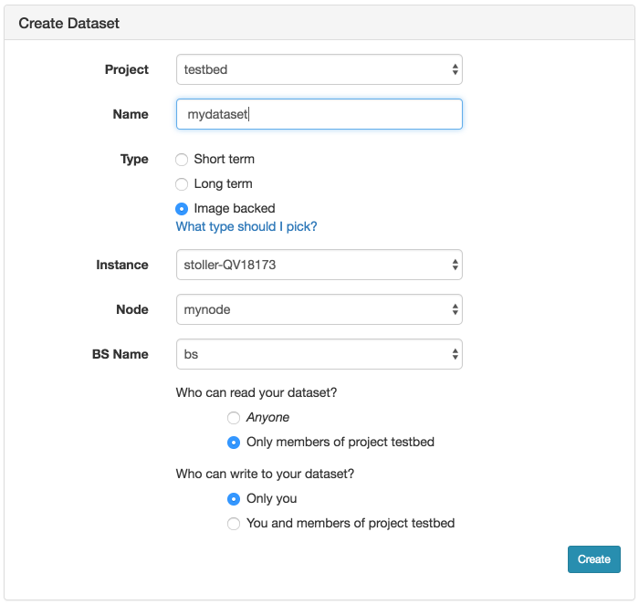
As shown, choose a name for your dataset and optionally the project the dataset should be associated with. Be sure to select Image Backed for the type. Then choose the experiment (Instance), which node in the experiment (Node), and which local dataset on the node (BS Name). The dataset name will be the first argument to the node.Blockstore method invocation in the profile used to create the local dataset (bs in the example above).
Before clicking the Create button, make sure that you have no processes running on the node and accessing the mounted filesystem. This might include processes logging to a file in that filesystem or your interactive shell if you are cd’ed to that directory. If you do not do this, the image creation will fail when it tries to unmount the filesystem to ensure a consistent snapshot.
After clicking Create, the process can take several minutes or longer, depending on the size of the file system. Progress will be displayed on the page:
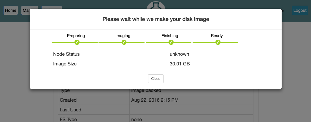
When the progress bar reaches the Ready stage, your new dataset is ready! It will now show up in your Storage drop-down under My Datasets and can be used in new experiments.
10.7.3 Using and Updating an Image-backed Dataset
To use an existing image-backed dataset, you will need to reference it in your profile, as demonstrated in:
"""An example of an image backed dataset. The dataset name and mountpoint can be customized when you instantiate the profile. Instructions: Log into your node, your dataset filesystem is in the directory you specified during profile instantiation.""" # Import the Portal object. import geni.portal as portal # Import the ProtoGENI library. import geni.rspec.pg as pg # Import the emulab extensions library. import geni.rspec.emulab # Create a portal context, needed to defined parameters pc = portal.Context() # Create a Request object to start building the RSpec. request = pc.makeRequestRSpec() pc.defineParameter("DATASET", "URN of your image-backed dataset", portal.ParameterType.STRING, "urn:publicid:IDN+emulab.net:testbed+imdataset+pgimdat") pc.defineParameter("MPOINT", "Mountpoint for file system", portal.ParameterType.STRING, "/mydata") params = pc.bindParameters() node = request.RawPC("mynode") node.disk_image = 'urn:publicid:IDN+emulab.net+image+emulab-ops//UBUNTU16-64-STD' bs = node.Blockstore("bs", params.MPOINT) bs.dataset = params.DATASET pc.printRequestRSpec(request)Open this profile on CloudLab"""An example of an image backed dataset. The dataset name and mountpoint can be customized when you instantiate the profile. Instructions: Log into your node, your dataset filesystem is in the directory you specified during profile instantiation.""" # Import the Portal object. import geni.portal as portal # Import the ProtoGENI library. import geni.rspec.pg as pg # Import the emulab extensions library. import geni.rspec.emulab # Create a portal context, needed to defined parameters pc = portal.Context() # Create a Request object to start building the RSpec. request = pc.makeRequestRSpec() pc.defineParameter("DATASET", "URN of your image-backed dataset", portal.ParameterType.STRING, "urn:publicid:IDN+emulab.net:testbed+imdataset+pgimdat") pc.defineParameter("MPOINT", "Mountpoint for file system", portal.ParameterType.STRING, "/mydata") params = pc.bindParameters() node = request.RawPC("mynode") node.disk_image = 'urn:publicid:IDN+emulab.net+image+emulab-ops//UBUNTU16-64-STD' bs = node.Blockstore("bs", params.MPOINT) bs.dataset = params.DATASET pc.printRequestRSpec(request)
This profile takes the dataset URN to use as a parameter during instantiation. You can find the URN for your dataset on the information page for the dataset. From the Storage drop-down, click on My Datasets, find the name of your dataset in the list, and click on it.
Once instantiated, the dataset will be accessible under /mydata (or whatever mountpoint you specified).
If you make changes and want to preserve them, you can update your dataset by using the Modify button on the My Datasets page for the dataset in question.
10.7.4 Creating a Remote Dataset
Creating a remote dataset is very similar to the process just described for creating an image-backed dataset. Click on the "Create Dataset" option in the Storage drop-down menu. This will bring up the form to create a new dataset:
Screenshot TBD
Choose a name for your dataset and optionally the project the dataset should be associated with.
Select Short term or Long term as the Type depending on your needs (click on “Which type should I pick” for more info).
Pick a Size, keeping in mind that sizes in excess of 1TB are likely to require administrative approval.
Pick the Cluster at which the dataset will be created. Recall that remote datasets are specific to a cluster and can only be used by nodes at that cluster.
If you selected a short-term dataset, you will need to fill in the expiration date (Expires), again keeping in mind that dates more than 1-2 weeks in the future will require administrative approval.
Pick the initial filesystem type you would like created on the dataset. Almost certainly you will want to use the default ext4. It is not necessary to create a filesystem (choose “none”) if you want to use the dataset as a raw disk or if you want to create your own filesystem on it when you first use it. Note however, if you do not choose a filesystem now, then you cannot set a mountpoint when you first use the dataset.
Finally, select the read and write permissions for the dataset.
After clicking Create, you may get a message informing you Your dataset needs to be approved! and giving you a reason why. If this is the case, your dataset will be shown as “unapproved” and you can either let it go and see if it is approved by CloudLab administrators, or you can Delete and try again with different parameters. (Note that Modify will only allow you to change the permission settings and cannot be used to alter the size or duration of the dataset.) The creation process can take several minutes or longer, depending on whether you specified a filesystem and what its size and type are.
Once it shows up in your My Datasets list as valid, you can use it in new experiments.
10.7.5 Using a Remote Dataset on a Single Node
Once you have created a remote dataset, you can make use of it in experiments. In many situations, you may only need to use the dataset on a single node. This is certainly the case after you have just created the dataset and need to populate it. This following profile demonstrates how to use a remote dataset:
"""This profile demonstrates how to use a remote dataset on your node, either a long term dataset or a short term dataset, created via the Portal. Instructions: Log into your node, your dataset file system in mounted at `/mydata`. """ # Import the Portal object. import geni.portal as portal # Import the ProtoGENI library. import geni.rspec.pg as rspec # Import the emulab extensions library. import geni.rspec.emulab # Create a Request object to start building the RSpec. request = portal.context.makeRequestRSpec() # Add a node to the request. node = request.RawPC("node") # We need a link to talk to the remote file system, so make an interface. iface = node.addInterface() # The remote file system is represented by special node. fsnode = request.RemoteBlockstore("fsnode", "/mydata") # This URN is displayed in the web interfaace for your dataset. fsnode.dataset = "urn:publicid:IDN+emulab.net:portalprofiles+ltdataset+DemoDataset" # # The "rwclone" attribute allows you to map a writable copy of the # indicated SAN-based dataset. In this way, multiple nodes can map # the same dataset simultaneously. In many situations, this is more # useful than a "readonly" mapping. For example, a dataset # containing a Linux source tree could be mapped into multiple # nodes, each of which could do its own independent, # non-conflicting configure and build in their respective copies. # Currently, rwclones are "ephemeral" in that any changes made are # lost when the experiment mapping the clone is terminated. # #fsnode.rwclone = True # # The "readonly" attribute, like the rwclone attribute, allows you to # map a dataset onto multiple nodes simultaneously. But with readonly, # those mappings will only allow read access (duh!) and any filesystem # (/mydata in this example) will thus be mounted read-only. Currently, # readonly mappings are implemented as clones that are exported # allowing just read access, so there are minimal efficiency reasons to # use a readonly mapping rather than a clone. The main reason to use a # readonly mapping is to avoid a situation in which you forget that # changes to a clone dataset are ephemeral, and then lose some # important changes when you terminate the experiment. # #fsnode.readonly = True # Now we add the link between the node and the special node fslink = request.Link("fslink") fslink.addInterface(iface) fslink.addInterface(fsnode.interface) # Special attributes for this link that we must use. fslink.best_effort = True fslink.vlan_tagging = True # Print the RSpec to the enclosing page. portal.context.printRequestRSpec()Open this profile on CloudLab"""This profile demonstrates how to use a remote dataset on your node, either a long term dataset or a short term dataset, created via the Portal. Instructions: Log into your node, your dataset file system in mounted at `/mydata`. """ # Import the Portal object. import geni.portal as portal # Import the ProtoGENI library. import geni.rspec.pg as rspec # Import the emulab extensions library. import geni.rspec.emulab # Create a Request object to start building the RSpec. request = portal.context.makeRequestRSpec() # Add a node to the request. node = request.RawPC("node") # We need a link to talk to the remote file system, so make an interface. iface = node.addInterface() # The remote file system is represented by special node. fsnode = request.RemoteBlockstore("fsnode", "/mydata") # This URN is displayed in the web interfaace for your dataset. fsnode.dataset = "urn:publicid:IDN+emulab.net:portalprofiles+ltdataset+DemoDataset" # # The "rwclone" attribute allows you to map a writable copy of the # indicated SAN-based dataset. In this way, multiple nodes can map # the same dataset simultaneously. In many situations, this is more # useful than a "readonly" mapping. For example, a dataset # containing a Linux source tree could be mapped into multiple # nodes, each of which could do its own independent, # non-conflicting configure and build in their respective copies. # Currently, rwclones are "ephemeral" in that any changes made are # lost when the experiment mapping the clone is terminated. # #fsnode.rwclone = True # # The "readonly" attribute, like the rwclone attribute, allows you to # map a dataset onto multiple nodes simultaneously. But with readonly, # those mappings will only allow read access (duh!) and any filesystem # (/mydata in this example) will thus be mounted read-only. Currently, # readonly mappings are implemented as clones that are exported # allowing just read access, so there are minimal efficiency reasons to # use a readonly mapping rather than a clone. The main reason to use a # readonly mapping is to avoid a situation in which you forget that # changes to a clone dataset are ephemeral, and then lose some # important changes when you terminate the experiment. # #fsnode.readonly = True # Now we add the link between the node and the special node fslink = request.Link("fslink") fslink.addInterface(iface) fslink.addInterface(fsnode.interface) # Special attributes for this link that we must use. fslink.best_effort = True fslink.vlan_tagging = True # Print the RSpec to the enclosing page. portal.context.printRequestRSpec()
You can find the URN for your dataset on the information page for the dataset. From the Storage drop-down, click on My Datasets, find the name of your dataset in the list, and click on it.
Note the “fslink” settings best_effort and vlan_tagging. These should always be set since some node types have only a single experimental interface. Since the remote dataset uses a network link and your experiment topology might also include a LAN with multiple nodes (see the following examples for multiple nodes), both uses will need to share the physical interface.
10.7.6 Using a Remote Dataset on Multiple Nodes via a Shared Filesystem
You cannot simply create a filesystem in a persistent remote dataset and directly share that among nodes in an experiment. If you want to share a standard Linux filesystem among nodes in an experiment, you can instead have one node in your experiment map the dataset read-write and have it act as an NFS server, exporting the dataset filesystem to all other nodes in the experiment via NFS on a shared LAN. This profile configures such an experiment with a variable number of client nodes:
"""This profile sets up a simple NFS server and a network of clients. The NFS server uses a long term dataset that is persistent across experiments. In order to use this profile, you will need to create your own dataset and use that instead of the demonstration dataset below. If you do not need persistant storage, we have another profile that uses temporary storage (removed when your experiment ends) that you can use. Instructions: Click on any node in the topology and choose the `shell` menu item. Your shared NFS directory is mounted at `/nfs` on all nodes.""" # Import the Portal object. import geni.portal as portal # Import the ProtoGENI library. import geni.rspec.pg as pg # Import the Emulab specific extensions. import geni.rspec.emulab as emulab # Create a portal context. pc = portal.Context() # Create a Request object to start building the RSpec. request = pc.makeRequestRSpec() # Only Ubuntu images supported. imageList = [ ('urn:publicid:IDN+emulab.net+image+emulab-ops//UBUNTU18-64-STD', 'UBUNTU 18.04'), ('urn:publicid:IDN+emulab.net+image+emulab-ops//UBUNTU16-64-STD', 'UBUNTU 16.04'), ('urn:publicid:IDN+emulab.net+image+emulab-ops//CENTOS7-64-STD', 'CENTOS 7'), ] # Do not change these unless you change the setup scripts too. nfsServerName = "nfs" nfsLanName = "nfsLan" nfsDirectory = "/nfs" # Number of NFS clients (there is always a server) pc.defineParameter("clientCount", "Number of NFS clients", portal.ParameterType.INTEGER, 2) pc.defineParameter("osImage", "Select OS image", portal.ParameterType.IMAGE, imageList[2], imageList) # Always need this when using parameters params = pc.bindParameters() # The NFS network. All these options are required. nfsLan = request.LAN(nfsLanName) nfsLan.best_effort = True nfsLan.vlan_tagging = True nfsLan.link_multiplexing = True # The NFS server. nfsServer = request.RawPC(nfsServerName) nfsServer.disk_image = params.osImage # Attach server to lan. nfsLan.addInterface(nfsServer.addInterface()) # Initialization script for the server nfsServer.addService(pg.Execute(shell="sh", command="sudo /bin/bash /local/repository/nfs-server.sh")) # Special node that represents the ISCSI device where the dataset resides dsnode = request.RemoteBlockstore("dsnode", nfsDirectory) dsnode.dataset = "urn:publicid:IDN+emulab.net:portalprofiles+ltdataset+DemoDataset" # Link between the nfsServer and the ISCSI device that holds the dataset dslink = request.Link("dslink") dslink.addInterface(dsnode.interface) dslink.addInterface(nfsServer.addInterface()) # Special attributes for this link that we must use. dslink.best_effort = True dslink.vlan_tagging = True dslink.link_multiplexing = True # The NFS clients, also attached to the NFS lan. for i in range(1, params.clientCount+1): node = request.RawPC("node%d" % i) node.disk_image = params.osImage nfsLan.addInterface(node.addInterface()) # Initialization script for the clients node.addService(pg.Execute(shell="sh", command="sudo /bin/bash /local/repository/nfs-client.sh")) pass # Print the RSpec to the enclosing page. pc.printRequestRSpec(request) """This profile sets up a simple NFS server and a network of clients. The NFS server uses a long term dataset that is persistent across experiments. In order to use this profile, you will need to create your own dataset and use that instead of the demonstration dataset below. If you do not need persistant storage, we have another profile that uses temporary storage (removed when your experiment ends) that you can use. Instructions: Click on any node in the topology and choose the `shell` menu item. Your shared NFS directory is mounted at `/nfs` on all nodes.""" # Import the Portal object. import geni.portal as portal # Import the ProtoGENI library. import geni.rspec.pg as pg # Import the Emulab specific extensions. import geni.rspec.emulab as emulab # Create a portal context. pc = portal.Context() # Create a Request object to start building the RSpec. request = pc.makeRequestRSpec() # Only Ubuntu images supported. imageList = [ ('urn:publicid:IDN+emulab.net+image+emulab-ops//UBUNTU18-64-STD', 'UBUNTU 18.04'), ('urn:publicid:IDN+emulab.net+image+emulab-ops//UBUNTU16-64-STD', 'UBUNTU 16.04'), ('urn:publicid:IDN+emulab.net+image+emulab-ops//CENTOS7-64-STD', 'CENTOS 7'), ] # Do not change these unless you change the setup scripts too. nfsServerName = "nfs" nfsLanName = "nfsLan" nfsDirectory = "/nfs" # Number of NFS clients (there is always a server) pc.defineParameter("clientCount", "Number of NFS clients", portal.ParameterType.INTEGER, 2) pc.defineParameter("osImage", "Select OS image", portal.ParameterType.IMAGE, imageList[2], imageList) # Always need this when using parameters params = pc.bindParameters() # The NFS network. All these options are required. nfsLan = request.LAN(nfsLanName) nfsLan.best_effort = True nfsLan.vlan_tagging = True nfsLan.link_multiplexing = True # The NFS server. nfsServer = request.RawPC(nfsServerName) nfsServer.disk_image = params.osImage # Attach server to lan. nfsLan.addInterface(nfsServer.addInterface()) # Initialization script for the server nfsServer.addService(pg.Execute(shell="sh", command="sudo /bin/bash /local/repository/nfs-server.sh")) # Special node that represents the ISCSI device where the dataset resides dsnode = request.RemoteBlockstore("dsnode", nfsDirectory) dsnode.dataset = "urn:publicid:IDN+emulab.net:portalprofiles+ltdataset+DemoDataset" # Link between the nfsServer and the ISCSI device that holds the dataset dslink = request.Link("dslink") dslink.addInterface(dsnode.interface) dslink.addInterface(nfsServer.addInterface()) # Special attributes for this link that we must use. dslink.best_effort = True dslink.vlan_tagging = True dslink.link_multiplexing = True # The NFS clients, also attached to the NFS lan. for i in range(1, params.clientCount+1): node = request.RawPC("node%d" % i) node.disk_image = params.osImage nfsLan.addInterface(node.addInterface()) # Initialization script for the clients node.addService(pg.Execute(shell="sh", command="sudo /bin/bash /local/repository/nfs-client.sh")) pass # Print the RSpec to the enclosing page. pc.printRequestRSpec(request)
10.7.7 Using a Remote Dataset on Multiple Nodes via Clones
TBD.
11 The Control Network
11.1 Overview
At every CloudLab cluster, the majority of the allocatable nodes (primarily general-purpose servers) are connected to a persistent, shared IPv4 subnet known as the control network. Each cluster has its own control network namespace, typically a subset of the affiliated university’s larger IPv4 namespace.
The control network at each cluster is used for two primary purposes. First, since it is Internet accessible, it provides the path through which users interact with their experiment nodes, including getting data in and out of CloudLab. Second, it is used by CloudLab infrastructure for experiment control. This includes initial imaging and configuration of nodes as well as ongoing monitoring of resource usage at the cluster level. It is also used for infrastructure coordination and control between the individual clusters and the master CloudLab portal at Utah.
The control network is distinct from the network topology connecting nodes as defined in an experiment’s profile. That topology, known as the experiment network, is realized at experiment instantiation time on a completely separate fabric of physical switches using vlans on those switches to implement an experiment’s links and lans. Each experiment network is isolated from those of other active experiments, and exists only for the lifetime of the experiment.
We do allow Internet wide experiments on occasion, but this requires permission from, and coordination with, CloudLab staff since such traffic tends to trigger monitors resulting in abuse reports from both at CloudLab host institutions and external sites.
The following sections elaborate on how to ensure your experiments use the correct network (including a list of common mistakes and how to empirically verify correct interface use), how to respond to a Control Network Violation message, why it is so important not to use the control network anyway, and finally after all the negativity, what activity is allowed on the control network.
11.2 Ensuring your experiment nodes use the correct interfaces
From the perspective of an experiment node, the control network and any experiment networks are accessed through the same OS-provided mechanisms. This requires that the experimenter know how to distinguish the two and ensure that they use the correct interfaces.
On the surface, the distinction is simple: active experiment interfaces will have 10.x.x.x private IPv4 addresses assigned to them. The control network interface will have an Internet routable IP address in the IANA-assigned IP space of the specific CloudLab cluster. All applications that transmit packets running on experiment nodes should use the 10.x.x.x addresses (or the aliases in /etc/hosts) when addressing other nodes in experiments. All applications listening for connections from other nodes in the experiment should bind to those names/addresses as well.
This sounds simple enough, but unfortunately there are a number of scenarios in which identifying the control interface is not so easy or it is not obvious that you are using it. The next section details some of the common mistakes made and how to avoid them.
11.2.1 Common causes of control network misuse
Use of a fully qualified domain name in applications. In CloudLab, fully qualified domain names (FQDN) for a node are mapped by the CloudLab DNS to the control network interface. This includes both the permanent “physical” node name assigned by the infrastructure (e.g., amd047.utah.cloudlab.us), and the ephemeral user-assigned virtual node name specified in the profile of an experiment instantiation (e.g., node1.myexpt.myproj.utah.cloudlab.us). Many applications, in particular Java applications, use the FQDN of a host to determine an IP address to use for “the network” resulting in its improper use of the control net. You will need to configure the application to explicitly use the “short name” of your experiment nodes in /etc/hosts or use the explicit 10.x.x.x IP address.
Using INADDR_ANY (0.0.0.0) for listening services. It is very common for applications that provide a network service to default to listening on every active interface via the INADDR_ANY address in a socket bind call. In CloudLab this will include the control network interface resulting in a service that is exposed to the Internet at large. While this is not directly a misuse of the control network, it becomes one if one of these services is compromised, as they often are due to weak security in the default configuration or due to known bugs. At this point compromised nodes often become part of a botnet launching attacks on other sites.
Fortunately, most applications include options to limit the interfaces on which they listen either by specifying those interfaces directly or by having an option to exclude specific interfaces.
Use of the wrong interface with RDMA and kernel-bypass networking. If your experimentation involves RDMA or other uses of highly optimized kernel-bypass network stacks (e.g., DPDK), you will need to make sure that your configuration of these tools is using the correct interface. In the case of RDMA, simply specifying an experiment network 10.x.x.x IP is often insufficient for ensuring your RDMA traffic flows over the correct interface. In utilities such as ib_send_bw for example, the internal IP is used for the handshake QP info exchange, but the physical port that it actually sends traffic out on is selected with a different argument. By default, it will select the first port on the first RDMA-capable NIC it finds, which will be the control network port on a number of CloudLab hardware types.
You will need to use utilities such as ibstat or ibv_devinfo to find the device that you actually want to send on, and then ensure that your application is properly configured to use that. In the case of ib_send_bw for example, you specify it with the -d command line argument.
Modifying the configuration of the control network interface. CloudLab infrastructure makes a number of assumptions about the control network namespace and bad things can happen if those assumptions are violated. Changing the IP address assigned to the control network interface, or removing it entirely, is obviously bad because the infrastructure and outside world can no longer talk to the node. Adding an alias to the interface can likewise cause problems. If you were to assign an additional routable IP address from a non-CloudLab network IP namespace, you are likely to trigger anti-spoofing measures at our gateway or beyond as non-CloudLab sourced packets get routed out of CloudLab. Even assigning a non-routable IP alias may have consequences as it could result in unintentional communication between your experiment node and another experiment’s nodes that happens to use an alias in the same subnet.
As a general rule, never change settings on the control network interface and ensure that applications do not do so either.
Unintentional use of the default route. The default route on CloudLab nodes is through the control network. This is necessary so that applications on nodes can communicate with arbitrary Internet hosts for SSH, DNS, and other well-behaved services.
For experiment network traffic, explicit routes via the experiment interfaces are added by the CloudLab software based on IP addresses explicitly or implicitly assigned in profiles. Thus use of any IP address other than these in your generated traffic, will cause that traffic to be routed using the default route via the control network. For example, replays of real world packet traces with routable IP destinations could result in sending packets with routable IP destinations out the control network, potentially wreaking havoc. Even simple typos when specifying 10.x.x.x addresses (e.g., using 10.2.1.1 in an app when you meant 10.1.1.1) will result in use of the default route. Use of IP multicast without a route for that traffic is another cause. Finally, disabling automatic route configuration in your experiment profile and attempting to setup the routing yourself, or forgetting to setup routing at all, is another common source of misrouting.
The best advise here is to let CloudLab handle IP assignment and route setup whenever possible and to verify that traffic is not going through the control network.
Use of the wrong interface when broadcasting or multicasting. Using the wrong interface for broadcast and multicast traffic can have much worse consequences than doing so for unicast traffic, so it is called out specially here.
Broadcasting packets on the control network interface of a node will effect every other active experiment node in the cluster as they must receive and ignore those packets adding unexpected and unwanted overhead. Likewise, every control network infrastructure switch must forward those packets on every active port. Given that even the oldest nodes in CloudLab can generate in excess of one million packets per second, the impact can be considerable. Certain types of multicast traffic can also cause issues when sent via the control network interface. In particular STP and IGMP packets that will be interpreted by the infrastructure switches.
Thus you must be extremely careful when using broadcast and multicast in an experiment. You should ensure that you have bound the traffic to the correct interface or that you have specified an explicit route for IP multicast.
Overuse of the infrastructure NFS filesystems. On each cluster, CloudLab provides a private, persistent NFS filesystem to every project. At any time, all nodes allocated to any experiment in project foo can access that space over the control network via /proj/foo.
This is a very convenient mechanism for providing a shared name space to all nodes in an experiment or across experiments. However, it should only be used for sporadic access to files and not for continuous reading and writing of datasets, databases, VM images, or log files to avoid overloading of the control network (and the infrastructure NFS server). This is especially a problem for large multi-node experiments simultaneously accessing the shared filesystem. See the storage section for alternatives to use for shared storage.
11.2.2 Empirically verifying interface use
It is always a good idea to ensure that your experiment is using the correct network interfaces after initial experiment setup has been done and once the involved applications are running. To do this you should start with the smallest instance of your experiment that is reasonable, just two nodes if possible, and then scale up to your desired size once you are confident that things are behaving correctly.
“Behaving correctly” in this context means “not using the control network excessively”, so we are only interested in getting a sense of the volume of traffic on the control network interface and whether there are any services listening on the interface that need not be. Following is a short list of techniques you can use to determine that.
Use the Graphs tab in the experiment status page. Every experiment node runs a monitoring daemon which collects resource usage as provided by the node OS. This information is reported (every five minutes) to the portal where it is aggregated and the results for all experiment nodes summarized on the Graphs tab. If the Control Traffic Graph shows over 100,000 packets-per-second, you are using the wrong interface. Only the Experiment Traffic Graph should show rates that high.
However, if you are using kernel-bypass networking (e.g., RDMA), then the OS-provided metrics will be wrong since the traffic is not passing through the kernel. In that case the Graphs tab will tell you nothing and you should try the Portstats tab.
Use the Portstats tab in the experiment status page. The Portstats data come from the infrastructure switches that a node’s control and experiment interfaces are connected to. Thus, it will still see traffic that the OS does not when using kernel-bypass. Unfortunately, Portstats data only show experiment network traffic, so this is at best an indirect metric; i.e., if there is a lot of experiment network traffic, the experiment is probably configured correctly. Note that the page also only displays the delta from the previous refresh, so the first call will show all experiment traffic from when the experiment was started. You will have to wait a few minutes and click the refresh icon to get a more meaningful reading. Also, not all control net switches support access to the switch counters, so you might not always get non-zero values from this tab.
Run tcpdump on the node. The Graphs tab will only give you an aggregate packet rate at five minute intervals. If you need to know more about the traffic or get an instantaneous snapshot, then you may be able to learn more using tcpdump. You need to be careful running on the control net interface however since you are likely logged into the node via ssh over the control network, and you do not want to capture your own interactions. Try:
tcpdump -c 500 -n -i ‘cat /var/emulab/boot/controlif‘ not port ssh and not arp
This will print out info about the first 500 packets it sees that are not from ssh (your login session) and are not ARP packets (we have a lot of normal ARP traffic on our control networks). If the command finishes nearly instantaneously and produces output too fast to read, then it is likely that something is sending or receiving at an abnormal rate. From the tcpdump output, you should be able to see the source and destination IP addresses and ports as well as the type of traffic. This may offer a clue as to what is happening.
Note that as with the Graphs tab, this method will not work with kernel-bypass network activity, tcpdump will not capture any of that traffic.
If you want to figure out if any of your experiment services are listening for connections on the control network, there are a couple of ways to test:
Try connecting to the service from another host. What “connecting” means is highly dependent on the service, but generally you can use telnet to attempt to connect to the service port. You should first try doing this from another CloudLab node using the target node’s control network IP address. If you can connect, then the service is definitely listening on the control network interface. This may still not be a problem, as the service might be blocked by the CloudLab firewall. You can try connecting to the service from your home or university machine as well. If you can connect, then the service is listening and likely exposed to the Internet at large. You should fix the configuration of the service to disable that interface or ensure that it is securely configured.
Run nmap on the experiment node. An nmap scan of your node will give you a good idea of all the ports (services) exposed from the node. Here it is better to run from outside of CloudLab as there are a number of services that are visible inside that do not pose a problem since they are blocked at the firewall. So if you have access to the nmap utility at your home location, then you can try scanning one of your experiment hosts using its FQDN. The only “open” service you should see is ssh (port 22).
Run lsof on server processes. You can use the lsof command, which should be installed on all supported CloudLab OS images, to see what ports a specific service (process) has open or do the same for all processes. Run:
sudo lsof -Pn -p PID | grep LISTEN
for a single process PID or:
sudo lsof -Pn | grep LISTEN
for all processes. if it shows *:portnum or IP:portnum where IP is the control network address, then it is listening on the control network.
This can be used with the remote method to determine which process is exposing a port.
11.3 What to do if you get a Control Network Violation email
There are two forms of “control network violations” that we send email notifications about. One is the “very unusual amount of traffic over the shared control network” message which is the result of our auto-detection of high traffic volumes (cluster-specific, but typically exceeding 1Gb/sec or 100,000 packets/sec) over an extended period of time (average over 10 minutes). The other is the “we have determined that one or more nodes in the experiment has been compromised” message which is usually the result of CloudLab staff receiving a message from the host site or an external administrator, that a CloudLab node is engaging in undesirable behavior.
In addition to sending the email, we may also:
freeze your CloudLab account, logging you out of the portal and blocking further logins.
quarantine your experiment, which entails rebooting all nodes in the experiment into a minimal Ubuntu Linux environment running from a RAM-based filesystem, collectively known as “the MFS”. The disk is left intact, allowing the experiment to resume later as though the nodes had just rebooted.
terminate your experiment, causing all nodes in the experiment to have their disks reloaded and returning them to the free pool. The experiment cannot be resumed.
In the high traffic volume case, we generally first send the email and wait for an hour or two for a response. If we get no response, we will freeze your account and quarantine your experiment. If we still get no response, we will terminate the experiment and leave your account frozen. Upon receiving a reply and reaching a resolution, we will unfreeze your account and release the experiment from quarantine, allowing the nodes to boot from disk again.
See Using the Recovery MFS for more information on accessing a quarantined node’s disk from the MFS.
Your responsibility as a user is first to make sure you whitelist email from CloudLab! We will only use email to reach out to you. It is not good to discover that your experiment has been terminated because you never saw email from us.
If you receive one of these emails from us, do not panic! In most instances, it is not a serious problem for us, just a situation that needs to be fixed. Even with compromised nodes, we understand that these things happen. If you make an honest effort to fix the problem and be diligent in future experiments, all is well. We want you to continue using CloudLab for your research!
Don’t panic, but do be responsible and respond quickly to the email so that the problem can be resolved quickly. Your initial response should include an explanation of what you are attempting to do, why that may have caused the problem observed, and what you plan to do to fix it.
We do make exceptions when the “excessive” traffic is necessary, or when a “compromised” node really isn’t.
11.4 Why is it so important to avoid the control network?
This document has been hammering home the point “Using the control network is bad!” while citing largely reasons why it causes problems for the CloudLab infrastructure. For example, high volumes of traffic (data or packet rate) can interfere with infrastructure services, in particular those that are UDP-based such as DHCP, TFTP and our multicast image distribution mechanism. This traffic can also affect other experiments, interfering with their interactions with the infrastructure or introducing overhead receiving and rejecting rogue traffic. This is exacerbated by the control net fabric not being as well provisioned as the experiment fabric: switches are typically 1Gb or 10Gb, having less interswitch bandwidth and being less balanced in the topology. The control network’s relative transparency to applications coupled with its accessibility from the Internet, makes it much easier to inadvertently run vulnerable services with insecure default security policies that are exposed more than intended. It also allows for running services that can hijack identical infrastructure services; e.g., ARP, DHCP, DNS, or NFS.
These are all reasons we as infrastructure providers care about. There are also good reasons that you as an experimenter should care. The experiment network fabric consists of higher bandwidth node NICs (10, 25, 100Gbps) coupled with better switches and higher bandwidth interconnects. This fabric provides isolation guarantees by using separate switch vlans per experiment link/lan and optional performance guarantees by not allowing over-provisioning of logical links onto the physical links. Together these provide a more reproducible environment for experimentation. Accidental use of the control network instead of the experiment network can undermine these characteristics. You might perform a benchmark expecting it to run over an isolated 100Gb link, but misconfiguration might cause it to use a 10Gb link over the shared network. Likewise a dynamic routing experiment over a carefully constructed multi-hop topology, might be circumvented by the routing daemons discovering and using the control network where all nodes are one hop from every other node.
11.5 When can I use the control network?
While there are many usage patterns of the control network you should avoid, there are times when it is legitimate to use it. These include:
Monitoring and control of nodes in an experiment.
Modest use of the shared NFS filesystem rooted at /proj, such as storage of gigabyte or smaller package tarballs that you install on nodes, or datasets that you reference infrequently.
Importing and exporting data at the start and end of experiments or transferring data between an expiring experiment instance and a new one, as long as you throttle the bandwidth when possible (scp -l or rsync –bwlimit).
In general, low bandwidth or one-time “bursty” use between CloudLab nodes and the Internet, or CloudLab nodes in one experiment to nodes in another experiment, are okay–think human interaction or 1Gb/sec or less of TCP traffic.
We are flexible however, so if you have a need to move a large amount of data in or out of CloudLab or between experiments quickly, just let us know in advance.
12 Advanced Topics
12.1 Disk Images
Most disk images in CloudLab are stored and distributed in the Frisbee disk image format. They are stored at block level, meaning that, in theory, any filesystem can be used. In practice, Frisbee’s filesystem-aware compression is used, which causes the image snapshotting and installation processes to parse the filesystem and skip free blocks; this provides large performance benefits and space savings. Frisbee has support for filesystems that are variants of the BSD UFS/FFS, Linux EXT, and Windows NTFS formats. The disk images created by Frisbee are bit-for-bit identical with the original image, with the caveat that free blocks are skipped and may contain leftover data from previous users.
Disk images in CloudLab are typically created by starting with one of CloudLab’s supplied images, customizing the contents, and taking a snapshot of the resulting disk. The snapshotting process reboots the node, as it boots into an MFS to ensure a quiescent disk. If you wish to bring in an image from outside of CloudLab or create a new one from scratch, please contact us for help; if this is a common request, we may add features to make it easier.
CloudLab has default disk image for each node type; after a node is freed by one experimenter, it is re-loaded with the default image before being released back into the free pool. As a result, profiles that use the default disk images typically instantiate faster than those that use custom images, as no disk loading occurs.
Frisbee loads disk images using a custom multicast protocol, so loading large numbers of nodes typically does not slow down the instantiation process much.
Images may be referred to in requests in three ways: by URN, by an unqualified name, and by URL. URNs refer to a specific image that may be hosted on any of the CloudLab-affilated clusters. An unqualified name refers to the version of the image hosted on the cluster on which the experiment is instantiated. If you have large images that CloudLab cannot store due to space constraints, you may host them yourself on a webserver and put the URL for the image into the profile. CloudLab will fetch your image on demand, and cache it for some period of time for efficient distribution.
Images in CloudLab are versioned, and CloudLab records the provenance of images. Image URLs and URNs can contain version numbers, in which case they refer to that specific version of the image, or they may omit the version number, in which case they refer to the latest version of the image at the time an experiment is instantiated.
12.2 RSpecs
The resources (nodes, links, etc.) that define a profile are expressed in the
RSpec
format from the GENI project. In general, RSpec should be thought of as a
sort of “assembly language”—
12.3 Public IP Access
CloudLab treats publicly-routable IP addresses as an allocatable resource.
By default, all physical hosts are given a public IP address. This IP address is determined by the host, rather than the experiment. There are two DNS names that point to this public address: a static one that is the node’s permanent hostname (such as pcXX.<cluster>.net), and a dynamic one that is assigned based on the experiment; this one may look like <vname>.<exp>.<proj>.<cluster>.net, where <vname> is the name assigned in the request RSpec, <eid> is the name assigned to the experiment, and proj is the project that the experiment belongs to. This name is predictable regardless of the physical nodes assigned.
By default, virtual machines are not given public IP addresses; basic remote access is provided through an ssh server running on a non-standard port, using the physical host’s IP address. This port can be discovered through the manifest of an instantiated experiment, or on the “list view” of the experiment page. If a public IP address is required for a virtual machine (for example, to host a webserver on it), a public address can be requested on a per-VM basis. If using the Jacks GUI, each VM has a checkbox to request a public address. If using python scripts and geni-lib, setting the routable_control_ip property of a node accomplishes the same effect. Different clusters will have different numbers of public addresses available for allocation in this manner.
12.3.1 Dynamic Public IP Addresses
In some cases, users would like to create their own virtual machines, and would like to give them public IP addresses. We also allow profiles to request a pool of dynamic addresses; VMs brought up by the user can then run DHCP to be assigned one of these addresses.
Profiles using python scripts and geni-lib can request dynamic IP address pools by constructing an AddressPool object (defined in the geni.rspec.igext module), as in the following example:
# Request a pool of 3 dynamic IP addresses pool = AddressPool( "poolname", 3 ) rspec.addResource( pool ) # Request a pool of 3 dynamic IP addresses pool = AddressPool( "poolname", 3 ) rspec.addResource( pool )
The addresses assigned to the pool are found in the experiment manifest.
12.4 Markdown
CloudLab supports Markdown in the major text fields in RSpecs. Markdown is a simple formatting syntax with a straightforward translation to basic HTML elements such as headers, lists, and pre-formatted text. You may find this useful in the description and instructions attached to your profile.
While editing a profile, you can preview the Markdown rendering of the Instructions or Description field by double-clicking within the text box.
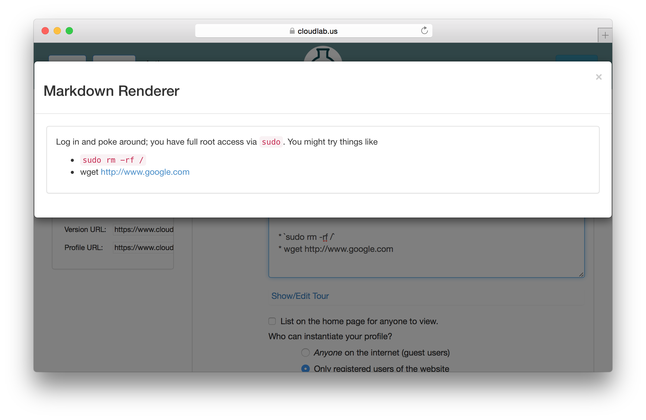
You will probably find the Markdown manual to be useful.
12.5 Introspection
CloudLab implements the GENI APIs, and in particular the geni-get command. geni-get is a generic means for nodes to query their own configuration and metadata, and is pre-installed on all facility-provided disk images. (If you are supplying your own disk image built from scratch, you can add the geni-get client from its repository.)
While geni-get supports many options, there are five commands most useful in the CloudLab context.
12.5.1 Client ID
Invoking geni-get client_id will print a single line to standard output showing the identifier specified in the profile corresponding to the node on which it is run. This is a particularly useful feature in execute services, where a script might want to vary its behaviour between different nodes.
12.5.2 Control MAC
The command geni-get control_mac will print the MAC address of the control interface (as a string of 12 hexadecimal digits with no punctuation). In some circumstances this can be a useful means to determine which interface is attached to the control network, as OSes are not necessarily consistent in assigning identifiers to network interfaces.
12.5.3 Manifest
To retrieve the manifest RSpec for the instance, you can use the command geni-get manifest. It will print the manifest to standard output, including any annotations added during instantiation. For instance, this is an appropriate technique to use to query the allocation of a dynamic public IP address pool.
12.5.4 Private key
As a convenience, CloudLab will automatically generate an RSA private key unique to each profile instance. geni-get key will retrieve the private half of the keypair, which makes it a useful command for profiles bootstraping an authenticated channel. For instance:
#!/bin/sh # Create the user SSH directory, just in case. mkdir $HOME/.ssh && chmod 700 $HOME/.ssh # Retrieve the server-generated RSA private key. geni-get key > $HOME/.ssh/id_rsa chmod 600 $HOME/.ssh/id_rsa # Derive the corresponding public key portion. ssh-keygen -y -f $HOME/.ssh/id_rsa > $HOME/.ssh/id_rsa.pub # If you want to permit login authenticated by the auto-generated key, # then append the public half to the authorized_keys2 file: grep -q -f $HOME/.ssh/id_rsa.pub $HOME/.ssh/authorized_keys2 || cat $HOME/.ssh/id_rsa.pub >> $HOME/.ssh/authorized_keys2 #!/bin/sh # Create the user SSH directory, just in case. mkdir $HOME/.ssh && chmod 700 $HOME/.ssh # Retrieve the server-generated RSA private key. geni-get key > $HOME/.ssh/id_rsa chmod 600 $HOME/.ssh/id_rsa # Derive the corresponding public key portion. ssh-keygen -y -f $HOME/.ssh/id_rsa > $HOME/.ssh/id_rsa.pub # If you want to permit login authenticated by the auto-generated key, # then append the public half to the authorized_keys2 file: grep -q -f $HOME/.ssh/id_rsa.pub $HOME/.ssh/authorized_keys2 || cat $HOME/.ssh/id_rsa.pub >> $HOME/.ssh/authorized_keys2
Please note that the private key will be accessible to any user who can invoke geni-get from within the profile instance. Therefore, it is NOT suitable for an authentication mechanism for privilege within a multi-user instance!
12.5.5 Profile parameters
When executing within the context of a profile instantiated with user-specified parameters, geni-get allows the retrieval of any of those parameters. The proper syntax is geni-get "param name", where name is the parameter name as specified in the geni-lib script defineParameter call. For example, geni-get "param n" would retrieve the number of nodes in an instance of the profile shown in the geni-lib parameter section.
12.6 User-controlled switches and layer-1 topologies
Some experiments require exclusive access to Ethernet switches and/or the ability for users to reconfigure those switches. One example of a good use case for this feature is to enable or tune QoS features that cannot be enabled on CloudLab’s shared infrastructure switches.
User-allocated switches are treated similarly to the way CloudLab treats servers: the switches appear as nodes in your topology, and you ’wire’ them to PCs and each other using point-to-point layer-1 links. When one of these switches is allocated to an experiment, that experiment is the exclusive user, just as it is for a raw PC, and the user has ssh access with full administrative control. This means that users are free to enable and disable features, tweak parameters, reconfigure as will, etc. Users are be given the switches in a ’clean’ state (we do little configuration on them), and can reload and reboot them like you would do with a server.
The list of available switches is found in our hardware chapter, and the following example shows how to request a simple topology using geni-lib.
"""This profile allocates two bare metal nodes and connects them together via a Dell or Mellanox switch with layer1 links. Instructions: Click on any node in the topology and choose the `shell` menu item. When your shell window appears, use `ping` to test the link. You will be able to ping the other node through the switch fabric. We have installed a minimal configuration on your switches that enables the ports that are in use, and turns on spanning-tree (RSTP) in case you inadvertently created a loop with your topology. All unused ports are disabled. The ports are in Vlan 1, which effectively gives a single broadcast domain. If you want anything fancier, you will need to open up a shell window to your switches and configure them yourself. If your topology has more then a single switch, and you have links between your switches, we will enable those ports too, but we do not put them into switchport mode or bond them into a single channel, you will need to do that yourself. If you make any changes to the switch configuration, be sure to write those changes to memory. We will wipe the switches clean and restore a default configuration when your experiment ends.""" # Import the Portal object. import geni.portal as portal # Import the ProtoGENI library. import geni.rspec.pg as pg # Import the Emulab specific extensions. import geni.rspec.emulab as emulab # Create a portal context. pc = portal.Context() # Create a Request object to start building the RSpec. request = pc.makeRequestRSpec() pc.defineParameter("phystype", "Switch type", portal.ParameterType.STRING, "dell-s4048", [('mlnx-sn2410', 'Mellanox SN2410'), ('dell-s4048', 'Dell S4048')]) # Retrieve the values the user specifies during instantiation. params = pc.bindParameters() # Do not run snmpit #request.skipVlans() # Add a raw PC to the request and give it an interface. node1 = request.RawPC("node1") iface1 = node1.addInterface() # Specify the IPv4 address iface1.addAddress(pg.IPv4Address("192.168.1.1", "255.255.255.0")) # Add Switch to the request and give it a couple of interfaces mysw = request.Switch("mysw"); mysw.hardware_type = params.phystype swiface1 = mysw.addInterface() swiface2 = mysw.addInterface() # Add another raw PC to the request and give it an interface. node2 = request.RawPC("node2") iface2 = node2.addInterface() # Specify the IPv4 address iface2.addAddress(pg.IPv4Address("192.168.1.2", "255.255.255.0")) # Add L1 link from node1 to mysw link1 = request.L1Link("link1") link1.addInterface(iface1) link1.addInterface(swiface1) # Add L1 link from node2 to mysw link2 = request.L1Link("link2") link2.addInterface(iface2) link2.addInterface(swiface2) # Print the RSpec to the enclosing page. pc.printRequestRSpec(request) Open this profile on CloudLab"""This profile allocates two bare metal nodes and connects them together via a Dell or Mellanox switch with layer1 links. Instructions: Click on any node in the topology and choose the `shell` menu item. When your shell window appears, use `ping` to test the link. You will be able to ping the other node through the switch fabric. We have installed a minimal configuration on your switches that enables the ports that are in use, and turns on spanning-tree (RSTP) in case you inadvertently created a loop with your topology. All unused ports are disabled. The ports are in Vlan 1, which effectively gives a single broadcast domain. If you want anything fancier, you will need to open up a shell window to your switches and configure them yourself. If your topology has more then a single switch, and you have links between your switches, we will enable those ports too, but we do not put them into switchport mode or bond them into a single channel, you will need to do that yourself. If you make any changes to the switch configuration, be sure to write those changes to memory. We will wipe the switches clean and restore a default configuration when your experiment ends.""" # Import the Portal object. import geni.portal as portal # Import the ProtoGENI library. import geni.rspec.pg as pg # Import the Emulab specific extensions. import geni.rspec.emulab as emulab # Create a portal context. pc = portal.Context() # Create a Request object to start building the RSpec. request = pc.makeRequestRSpec() pc.defineParameter("phystype", "Switch type", portal.ParameterType.STRING, "dell-s4048", [('mlnx-sn2410', 'Mellanox SN2410'), ('dell-s4048', 'Dell S4048')]) # Retrieve the values the user specifies during instantiation. params = pc.bindParameters() # Do not run snmpit #request.skipVlans() # Add a raw PC to the request and give it an interface. node1 = request.RawPC("node1") iface1 = node1.addInterface() # Specify the IPv4 address iface1.addAddress(pg.IPv4Address("192.168.1.1", "255.255.255.0")) # Add Switch to the request and give it a couple of interfaces mysw = request.Switch("mysw"); mysw.hardware_type = params.phystype swiface1 = mysw.addInterface() swiface2 = mysw.addInterface() # Add another raw PC to the request and give it an interface. node2 = request.RawPC("node2") iface2 = node2.addInterface() # Specify the IPv4 address iface2.addAddress(pg.IPv4Address("192.168.1.2", "255.255.255.0")) # Add L1 link from node1 to mysw link1 = request.L1Link("link1") link1.addInterface(iface1) link1.addInterface(swiface1) # Add L1 link from node2 to mysw link2 = request.L1Link("link2") link2.addInterface(iface2) link2.addInterface(swiface2) # Print the RSpec to the enclosing page. pc.printRequestRSpec(request)
This feature is implemented using a set of layer-1 switches between some servers and Ethernet switches. These switches act as “patch panels,” allowing us to “wire” servers to switches with no intervening Ethernet packet processing and minimal impact on latency. This feature can also be used to “wire” servers directly to one another, and to create links between switches, as seen in the following two examples.
"""This profile allocates two bare metal nodes and connects them directly together via a layer1 link. Instructions: Click on any node in the topology and choose the `shell` menu item. When your shell window appears, use `ping` to test the link.""" # Import the Portal object. import geni.portal as portal # Import the ProtoGENI library. import geni.rspec.pg as pg # Import the Emulab specific extensions. import geni.rspec.emulab as emulab # Create a portal context. pc = portal.Context() # Create a Request object to start building the RSpec. request = pc.makeRequestRSpec() # Do not run snmpit #request.skipVlans() # Add a raw PC to the request and give it an interface. node1 = request.RawPC("node1") # Must use UBUNTU18 to utilize layer 1 links. node1.disk_image = "urn:publicid:IDN+emulab.net+image+emulab-ops//UBUNTU18-64-STD" iface1 = node1.addInterface() # Specify the IPv4 address iface1.addAddress(pg.IPv4Address("192.168.1.1", "255.255.255.0")) # Add another raw PC to the request and give it an interface. node2 = request.RawPC("node2") # Must use UBUNTU18 to utilize layer 1 links. node2.disk_image = "urn:publicid:IDN+emulab.net+image+emulab-ops//UBUNTU18-64-STD" iface2 = node2.addInterface() # Specify the IPv4 address iface2.addAddress(pg.IPv4Address("192.168.1.2", "255.255.255.0")) # Add L1 link from node1 to node2 link1 = request.L1Link("link1") link1.addInterface(iface1) link1.addInterface(iface2) # Print the RSpec to the enclosing page. pc.printRequestRSpec(request) Open this profile on CloudLab"""This profile allocates two bare metal nodes and connects them directly together via a layer1 link. Instructions: Click on any node in the topology and choose the `shell` menu item. When your shell window appears, use `ping` to test the link.""" # Import the Portal object. import geni.portal as portal # Import the ProtoGENI library. import geni.rspec.pg as pg # Import the Emulab specific extensions. import geni.rspec.emulab as emulab # Create a portal context. pc = portal.Context() # Create a Request object to start building the RSpec. request = pc.makeRequestRSpec() # Do not run snmpit #request.skipVlans() # Add a raw PC to the request and give it an interface. node1 = request.RawPC("node1") # Must use UBUNTU18 to utilize layer 1 links. node1.disk_image = "urn:publicid:IDN+emulab.net+image+emulab-ops//UBUNTU18-64-STD" iface1 = node1.addInterface() # Specify the IPv4 address iface1.addAddress(pg.IPv4Address("192.168.1.1", "255.255.255.0")) # Add another raw PC to the request and give it an interface. node2 = request.RawPC("node2") # Must use UBUNTU18 to utilize layer 1 links. node2.disk_image = "urn:publicid:IDN+emulab.net+image+emulab-ops//UBUNTU18-64-STD" iface2 = node2.addInterface() # Specify the IPv4 address iface2.addAddress(pg.IPv4Address("192.168.1.2", "255.255.255.0")) # Add L1 link from node1 to node2 link1 = request.L1Link("link1") link1.addInterface(iface1) link1.addInterface(iface2) # Print the RSpec to the enclosing page. pc.printRequestRSpec(request)
"""This profile allocates two bare metal nodes and connects them together via two Dell or Mellanox switches with layer1 links. Instructions: Click on any node in the topology and choose the `shell` menu item. When your shell window appears, use `ping` to test the link. You will be able to ping the other node through the switch fabric. We have installed a minimal configuration on your switches that enables the ports that are in use, and turns on spanning-tree (RSTP) in case you inadvertently created a loop with your topology. All unused ports are disabled. The ports are in Vlan 1, which effectively gives a single broadcast domain. If you want anything fancier, you will need to open up a shell window to your switches and configure them yourself. If your topology has more then a single switch, and you have links between your switches, we will enable those ports too, but we do not put them into switchport mode or bond them into a single channel, you will need to do that yourself. If you make any changes to the switch configuration, be sure to write those changes to memory. We will wipe the switches clean and restore a default configuration when your experiment ends.""" # Import the Portal object. import geni.portal as portal # Import the ProtoGENI library. import geni.rspec.pg as pg # Import the Emulab specific extensions. import geni.rspec.emulab as emulab # Create a portal context. pc = portal.Context() # Create a Request object to start building the RSpec. request = pc.makeRequestRSpec() pc.defineParameter("phystype1", "Switch 1 type", portal.ParameterType.STRING, "dell-s4048", [('mlnx-sn2410', 'Mellanox SN2410'), ('dell-s4048', 'Dell S4048')]) pc.defineParameter("phystype2", "Switch 2 type", portal.ParameterType.STRING, "dell-s4048", [('mlnx-sn2410', 'Mellanox SN2410'), ('dell-s4048', 'Dell S4048')]) # Retrieve the values the user specifies during instantiation. params = pc.bindParameters() # Do not run snmpit #request.skipVlans() # Add a raw PC to the request and give it an interface. node1 = request.RawPC("node1") iface1 = node1.addInterface() # Specify the IPv4 address iface1.addAddress(pg.IPv4Address("192.168.1.1", "255.255.255.0")) # Add first switch to the request and give it a couple of interfaces mysw1 = request.Switch("mysw1"); mysw1.hardware_type = params.phystype1 sw1iface1 = mysw1.addInterface() sw1iface2 = mysw1.addInterface() # Add second switch to the request and give it a couple of interfaces mysw2 = request.Switch("mysw2"); mysw2.hardware_type = params.phystype2 sw2iface1 = mysw2.addInterface() sw2iface2 = mysw2.addInterface() # Add another raw PC to the request and give it an interface. node2 = request.RawPC("node2") iface2 = node2.addInterface() # Specify the IPv4 address iface2.addAddress(pg.IPv4Address("192.168.1.2", "255.255.255.0")) # Add L1 link from node1 to mysw1 link1 = request.L1Link("link1") link1.addInterface(iface1) link1.addInterface(sw1iface1) # Add L1 link from mysw1 to mysw2 trunk = request.L1Link("trunk") trunk.addInterface(sw1iface2) trunk.addInterface(sw2iface2) # Add L1 link from node2 to mysw2 link2 = request.L1Link("link2") link2.addInterface(iface2) link2.addInterface(sw2iface1) # Print the RSpec to the enclosing page. pc.printRequestRSpec(request) Open this profile on CloudLab"""This profile allocates two bare metal nodes and connects them together via two Dell or Mellanox switches with layer1 links. Instructions: Click on any node in the topology and choose the `shell` menu item. When your shell window appears, use `ping` to test the link. You will be able to ping the other node through the switch fabric. We have installed a minimal configuration on your switches that enables the ports that are in use, and turns on spanning-tree (RSTP) in case you inadvertently created a loop with your topology. All unused ports are disabled. The ports are in Vlan 1, which effectively gives a single broadcast domain. If you want anything fancier, you will need to open up a shell window to your switches and configure them yourself. If your topology has more then a single switch, and you have links between your switches, we will enable those ports too, but we do not put them into switchport mode or bond them into a single channel, you will need to do that yourself. If you make any changes to the switch configuration, be sure to write those changes to memory. We will wipe the switches clean and restore a default configuration when your experiment ends.""" # Import the Portal object. import geni.portal as portal # Import the ProtoGENI library. import geni.rspec.pg as pg # Import the Emulab specific extensions. import geni.rspec.emulab as emulab # Create a portal context. pc = portal.Context() # Create a Request object to start building the RSpec. request = pc.makeRequestRSpec() pc.defineParameter("phystype1", "Switch 1 type", portal.ParameterType.STRING, "dell-s4048", [('mlnx-sn2410', 'Mellanox SN2410'), ('dell-s4048', 'Dell S4048')]) pc.defineParameter("phystype2", "Switch 2 type", portal.ParameterType.STRING, "dell-s4048", [('mlnx-sn2410', 'Mellanox SN2410'), ('dell-s4048', 'Dell S4048')]) # Retrieve the values the user specifies during instantiation. params = pc.bindParameters() # Do not run snmpit #request.skipVlans() # Add a raw PC to the request and give it an interface. node1 = request.RawPC("node1") iface1 = node1.addInterface() # Specify the IPv4 address iface1.addAddress(pg.IPv4Address("192.168.1.1", "255.255.255.0")) # Add first switch to the request and give it a couple of interfaces mysw1 = request.Switch("mysw1"); mysw1.hardware_type = params.phystype1 sw1iface1 = mysw1.addInterface() sw1iface2 = mysw1.addInterface() # Add second switch to the request and give it a couple of interfaces mysw2 = request.Switch("mysw2"); mysw2.hardware_type = params.phystype2 sw2iface1 = mysw2.addInterface() sw2iface2 = mysw2.addInterface() # Add another raw PC to the request and give it an interface. node2 = request.RawPC("node2") iface2 = node2.addInterface() # Specify the IPv4 address iface2.addAddress(pg.IPv4Address("192.168.1.2", "255.255.255.0")) # Add L1 link from node1 to mysw1 link1 = request.L1Link("link1") link1.addInterface(iface1) link1.addInterface(sw1iface1) # Add L1 link from mysw1 to mysw2 trunk = request.L1Link("trunk") trunk.addInterface(sw1iface2) trunk.addInterface(sw2iface2) # Add L1 link from node2 to mysw2 link2 = request.L1Link("link2") link2.addInterface(iface2) link2.addInterface(sw2iface1) # Print the RSpec to the enclosing page. pc.printRequestRSpec(request)
12.7 Portal API
The CloudLab portal provides an API that makes it possible to programmatically instantiate, interact with, and terminate experiments.
We provide a Python client library containing both programmatic API bindings and an interactive CLI tool: see https://gitlab.flux.utah.edu/emulab/portal-api. Its README file provides comprehensive instruction on installation and usage. We also provide auto-generated API documentation built from the OpenAPI description that includes both CLI and Python examples for each RESTful endpoint.
The Portal API is under active development, so please let us know (see the Getting Help section) if an existing feature you need is not yet exposed in the API.
12.8 Legacy Portal API
The legacy Portal API should be considered deprecated.
We provide a Python library to interact with the legacy XMLRPC Portal API: see https://gitlab.flux.utah.edu/stoller/portal-tools. Its README file provides comprehensive instruction on usage, and the repository also contains an API description.
13 Hardware
CloudLab can allocate experiments on any one of several federated clusters.
CloudLab has the ability to dispatch experiments to several clusters: three that belong to CloudLab itself, plus several more that belong to federated projects.
Additional information about these nodes can be found at https://www.cloudlab.us/portal-hardware.php
13.1 CloudLab Utah
The CloudLab cluster at the University of Utah is being built in partnership with HP and Dell. It currently consists of 4 Intel Ice Lake servers, 208 AMD EPYC Rome servers (two generations), 170 Intel Xeon E5 servers, 270 Xeon-D servers, and 270 64-bit ARM servers for a total of 9,336 cores. The cluster is housed in the University of Utah’s Downtown Data Center in Salt Lake City.
m400 |
| 45 nodes (64-bit ARM) |
CPU |
| Eight 64-bit ARMv8 (Atlas/A57) cores at 2.4 GHz (APM X-GENE) |
RAM |
| 64GB ECC Memory (8x 8 GB DDR3-1600 SO-DIMMs) |
Disk |
| 120 GB of flash (SATA3 / M.2, Micron M500) |
NIC |
| Dual-port Mellanox ConnectX-3 10 GB NIC (PCIe v3.0, 8 lanes (one port available for experiment use) |
m510 |
| 270 nodes (Intel Xeon-D) |
CPU |
| Eight-core Intel Xeon D-1548 at 2.0 GHz |
RAM |
| 64GB ECC Memory (4x 16 GB DDR4-2133 SO-DIMMs) |
Disk |
| 256 GB NVMe flash storage |
NIC |
| Dual-port Mellanox ConnectX-3 10 GB NIC (PCIe v3.0, 8 lanes (one port available for experiment use) |
For the m400 and m510 node types, there are 45 nodes in a chassis with a total of seven chassis. Each chassis has two 45XGc switches; each node is connected to both switches. One switch is used for control traffic, connecting to the Internet, etc. The other is used to build experiment topologies, and should be used for most experimental purposes. Each chassis switch has four 40Gbps uplinks, the control net switch uplinks with a single 40Gb connection while the experiment net has three 40Gb uplinks.
Upon request and with help from CloudLab staff, users can allocate an entire chassis. When allocated in this mode, it is possible to have complete administrator control over the experiment switch in addition to the nodes.
In phase two we added 50 Apollo R2200 chassis each with four HPE ProLiant XL170r server modules. Each server has 10 cores for a total of 2000 cores.
xl170 |
| 200 nodes (Intel Broadwell, 10 core, 1 disk) |
CPU |
| Ten-core Intel E5-2640v4 at 2.4 GHz |
RAM |
| 64GB ECC Memory (4x 16 GB DDR4-2400 DIMMs) |
Disk |
| Intel DC S3520 480 GB 6G SATA SSD |
NIC |
| Two Dual-port Mellanox ConnectX-4 25 GB NIC (PCIe v3.0, 8 lanes (two ports available for experiment use, one 10Gb and one 25Gb) |
Each server is connected via a 10Gbps control link (Dell switches) and a 25Gbps experimental link to Mellanox 2410 switches in groups of 40 servers. Each of the five groups’ experimental switches are connected to a Mellanox 2700 spine switch at 5x100Gbps. That switch in turn interconnects with the rest of the Utah CloudLab cluster via 6x40Gbps uplinks to the HP FlexFabric 12910 switch.
A unique feature of the phase two nodes is the addition of eight ONIE bootable "user allocatable" switches that can run a variety of Open Network OSes: six Dell S4048-ONs and two Mellanox MSN2410-BB2Fs. These switches and all 200 nodes are connected to two NetScout 3903 layer-1 switches, allowing flexible combinations of nodes and switches in an experiment. Note that links through the NetScout switches are only 10Gb, not 25Gb.
For phase two we also added 28 Dell AMD EPYC-based servers with dual 100Gb Ethernet ports.
d6515 |
| 28 nodes (AMD EPYC Rome, 32 core, 2 disk, 100Gb Ethernet) |
CPU |
| 32-core AMD 7452 at 2.35GHz |
RAM |
| 128GB ECC Memory (8x 16 GB 3200MT/s RDIMMs) |
Disk |
| Two 480 GB 6G SATA SSD |
NIC |
| Dual-port Mellanox ConnectX-5 100 GB NIC (PCIe v4.0) (both ports available for experiment use) |
NIC |
| Dual-port Broadcom 57414 25 GB NIC (one port available for experiment use) |
Each server is connected via a 25Gbps control link (Dell S5224F switch), 2 x 100Gbs experiment links (Dell Z9264F-ON switch), and a 25Gbps experiment link (Dell S5248F-ON switch). The experiment switches are connected to the "phase two" Mellanox 2700 spine switch at 4x100Gbps (Z9264F) and 2x100Gbps (S5248F).
In the initial installment of phase three (2021) we added 180 more AMD EPYC Rome servers in two configurations.
c6525-25g |
| 144 nodes (AMD EPYC Rome, 16 core, 2 disk, 25Gb Ethernet) |
CPU |
| 16-core AMD 7302P at 3.00GHz |
RAM |
| 128GB ECC Memory (8x 16 GB 3200MT/s RDIMMs) |
Disk |
| Two 480 GB 6G SATA SSD |
NIC |
| Two dual-port Mellanox ConnectX-5 25Gb GB NIC (PCIe v4.0) (two ports available for experiment use) |
c6525-100g |
| 36 nodes (AMD EPYC Rome, 24 core, 2 disk, 25/100Gb Ethernet) |
CPU |
| 24-core AMD 7402P at 2.80GHz |
RAM |
| 128GB ECC Memory (8x 16 GB 3200MT/s RDIMMs) |
Disk |
| Two 1.6 TB NVMe SSD (PCIe v4.0) |
NIC |
| Dual-port Mellanox ConnectX-5 25 GB NIC (PCIe v4.0) (one port available for experiment use) |
NIC |
| Dual-port Mellanox ConnectX-5 Ex 100 GB NIC (PCIe v4.0) (one port available for experiment use) |
The "-25g" variant nodes have 2 x 25Gb experiment links (Dell S5296F switches) and SATA-based SSDs, and are intended for general experimentation.
The "-100g" variant nodes have one 25Gb (Dell S5296) and one 100Gb (Dell Z9264) experiment link as well as two large NVMe-based SSDs and more cores, and are intended for network and storage intensive experimentation.
Each server is also connected via a 25Gbps control link (Dell S5296F switch).
The experiment switches are interconnected via a single Dell Z9332 using 4-8 100Gb links each.
In the second installment of phase three (early 2022), we added a small set of "expandable" nodes, 2U boxes with multiple PCIe slots available for add in devices such as GPUs, FPGA, or other accelerator cards.
d750 |
| 4 nodes (Intel Ice Lake, 16 core, 2 disk, 25Gb Ethernet) |
CPU |
| 16-core Intel Xeon Gold 6326 at 2.90GHz |
RAM |
| 128GB ECC Memory (16x 8 GB 3200MT/s RDIMMs) |
Disk |
| 480 GB SATA SSD (PCIe v4.0) |
Disk |
| 400 GB NVMe Optane P5800X SSD (PCIe v4.0) |
NIC |
| Quad-port BCM57504 NetXtreme-E 25 GB NIC (three ports available for experiment use) |
Each server is also connected via a 25Gbps control link (Dell S5296F switch) and three 25Gbps experiment links (via another Dell S5296F switch).
These machines have four available full-length double-wide PCIe v4 x16 slots and 2400W power supplies capable of handling four enterprise GPUs or other accelerator cards.
They also have a 400GB Optane write-intensive SSD providing another level of storage hierarchy for experimentation.
NOTE: due to the small number of these nodes and their specialized hardware, they are not available for general use. CloudLab staff will grant access to your project on request. Be sure to include the type, your project and your reason for needing the specific type in your request.
Phase four (early 2025) focuses primarily on adding large scale 100Gb connectivity and more expandable nodes with an emphasis on Intel processors.
The 100Gb nodes are chassis-based Dell C6620 nodes:
c6620 |
| 132 nodes (Intel Emerald Rapids, 28 core, 2 disk, 25Gb+100Gb Ethernet) |
CPU |
| 28-core Intel Xeon Gold 5512U at 2.1GHz |
RAM |
| 128GB ECC Memory (8x 16 GB 5600MT/s RDIMMs) |
Disk |
| Two 800 GB Mixed-use Gen4 NVMe SSD |
NIC |
| Dual-port Intel E810-XXV 25Gb NIC (one port available for experiment use) |
NIC |
| Dual-port Intel E810-C 100Gb NIC (one port available for experiment use) |
There are three new types of "expandable" nodes:
d7615 |
| 6 nodes (AMD EPYC, 32 core, 3 disk, 25/100Gb Ethernet) |
CPU |
| 32-core AMD EPYC 9354P at 3.25GHz |
RAM |
| 192GB ECC Memory (12x 16 GB 5600MT/s RDIMMs) |
Disk |
| 480 GB NVMe SSD (BOSS-N1 controller) |
Disk |
| Two 1.6TB NVMe SSD (PCIe v5.0) |
NIC |
| Dual-port Mellanox ConnectX-6 Lx 25Gb NIC (one port available for experiment use) |
NIC |
| Dual-port Mellanox ConnectX-6 DX 100Gb NIC (one port available for experiment use) |
d760 |
| 4 nodes (Intel Emerald Rapids, 64 core, 3 disk, 25/100Gb Ethernet) |
CPU |
| Two 32-core Intel Xeon Gold 6548Y+ at 2.50GHz |
RAM |
| 256GB ECC Memory (16x 16 GB 5600MT/s RDIMMs) |
Disk |
| 480 GB NVMe SSD (BOSS-N1 controller) |
Disk |
| Two 1.6TB NVMe SSD (PCIe v5.0) |
NIC |
| Dual-port Intel E810-XXV 25Gb NIC (one port available for experiment use) |
NIC |
| Dual-port Intel E810-C 100Gb NIC (one port available for experiment use) |
d760-hbm |
| 2 nodes (Intel Emerald Rapids with high bandwidth memory, 64 core, 3 disk, 25/100Gb Ethernet) |
CPU |
| Two 32-core Intel Xeon Max 9462 at 2.70GHz |
HBM |
| 64GB per CPU |
RAM |
| 256GB ECC Memory (16x 16 GB 5600MT/s RDIMMs) |
Disk |
| 480 GB NVMe SSD (BOSS-N1 controller) |
Disk |
| Two 1.6TB NVMe SSD (PCIe v5.0) |
NIC |
| Dual-port Intel E810-XXV 25Gb NIC (one port available for experiment use) |
NIC |
| Dual-port Intel E810-C 100Gb NIC (one port available for experiment use) |
NOTE: due to the small number of these nodes and their specialized hardware, they are not available for general use. CloudLab staff will grant access to your project on request. Be sure to include the type, your project, and your reason for needing the specific type in your request.
All Phase four nodes are connected via a 25Gbps control link (Dell S5296F switch), one 25Gbps experiment link (via one of two other Dell S5296F switches), and one 100Gbps experiment link (all on a single Dell Z9664F switch).
The expandable machines have available PCIe gen4 and gen5 slots and 2400W power supplies capable of handling enterprise GPUs or other accelerator cards.
The Utah Cloudlab cluster includes a storage server for remote datasets. The server currently has 500TB available for allocation.
13.2 CloudLab Wisconsin
The CloudLab cluster at the University of Wisconsin is built in partnership with Cisco, Seagate, and HP. The cluster, which is in Madison, Wisconsin, has 568 servers with a total of 11,412 cores connected in a CLOS topology with full bisection bandwidth. It has 1,574 TB of storage, including SSDs on most nodes.
NOTE: In Early 2024 the c220g5, c240g5, and c4130 nodes had their experiment networking redone. c220g5 nodes now have 2x10Gb links (up from one link), c240g5s have 2x25Gb (up from 2x10Gb), and the c4130s have 2x100Gb (up from 2x10Gb). The changes are reflected below.
c220g1 |
| 88 nodes (Haswell, 16 core, 3 disks) |
CPU |
| Two Intel E5-2630 v3 8-core CPUs at 2.40 GHz (Haswell w/ EM64T) |
RAM |
| 128GB ECC Memory (8x 16 GB DDR4 1866 MHz dual rank RDIMMs) |
Disk |
| Two 1.2 TB 10K RPM 6G SAS SFF HDDs |
Disk |
| One Intel DC S3500 480 GB 6G SATA SSDs |
NIC |
| Dual-port Intel X520-DA2 10Gb NIC (PCIe v3.0, 8 lanes) (both ports available for experiment use) |
NIC |
| Onboard Intel i350 1Gb |
c240g1 |
| 5 nodes (Haswell, 16 core, 14 disks) |
CPU |
| Two Intel E5-2630 v3 8-core CPUs at 2.40 GHz (Haswell w/ EM64T) |
RAM |
| 128GB ECC Memory (8x 16 GB DDR4 1866 MHz dual rank RDIMMs) |
Disk |
| Two Intel DC S3500 480 GB 6G SATA SSDs |
Disk |
| Twelve 3 TB HDDs donated by Seagate |
NIC |
| Dual-port Intel X520-DA2 10Gb NIC (PCIe v3.0, 8 lanes) (both ports available for experiment use) |
NIC |
| Onboard Intel i350 1Gb |
c220g2 |
| 159 nodes (Haswell, 20 core, 3 disks) |
CPU |
| Two Intel E5-2660 v3 10-core CPUs at 2.60 GHz (Haswell EP) |
RAM |
| 160GB ECC Memory (10x 16 GB DDR4 2133 MHz dual rank RDIMMs) |
Disk |
| One Intel DC S3500 480 GB 6G SATA SSDs |
Disk |
| Two 1.2 TB 10K RPM 6G SAS SFF HDDs |
NIC |
| Dual-port Intel X520 10Gb NIC (PCIe v3.0, 8 lanes) (both ports available for experiment use) |
NIC |
| Onboard Intel i350 1Gb |
c240g2 |
| 3 nodes (Haswell, 20 core, 8 disks) |
CPU |
| Two Intel E5-2660 v3 10-core CPUs at 2.60 GHz (Haswell EP) |
RAM |
| 160GB ECC Memory (10x 16 GB DDR4 2133 MHz dual rank RDIMMs) |
Disk |
| Two Intel DC S3500 480 GB 6G SATA SSDs |
Disk |
| Two 1TB HDDs |
Disk |
| Four 3TB HDDs |
NIC |
| Dual-port Intel X520 10Gb NIC (PCIe v3.0, 8 lanes) (both ports available for experiment use) |
NIC |
| Onboard Intel i350 1Gb |
Phase two added 260 new nodes, 36 with one or more GPUs:
c220g5 |
| 219 nodes (Intel Skylake, 20 core, 2 disks) |
CPU |
| Two Intel Xeon Silver 4114 10-core CPUs at 2.20 GHz |
RAM |
| 192GB ECC DDR4-2666 Memory |
Disk |
| One 1 TB 7200 RPM 6G SAS HDs |
Disk |
| One Intel DC S3500 480 GB 6G SATA SSD |
NIC |
| Dual-port Intel X520-DA2 10Gb NIC (PCIe v3.0, 8 lanes) (both ports available for experiment use) |
NIC |
| Onboard Intel i350 1Gb |
c240g5 |
| 32 nodes (Intel Skylake, 20 core, 2 disks, GPU) |
CPU |
| Two Intel Xeon Silver 4114 10-core CPUs at 2.20 GHz |
RAM |
| 192GB ECC DDR4-2666 Memory |
Disk |
| One 1 TB 7200 RPM 6G SAS HDs |
Disk |
| One Intel DC S3500 480 GB 6G SATA SSD |
GPU |
| One NVIDIA 12GB PCI P100 GPU |
NIC |
| Dual-port Mellanox 25Gb NIC (PCIe v3.0, 8 lanes) (both ports available for experiment use) |
NIC |
| Onboard Intel i350 1Gb |
c4130 |
| 4 nodes (Intel Broadwell, 16 core, 2 disks, 4 GPUs) |
CPU |
| Two Intel Xeon E5-2667 8-core CPUs at 3.20 GHz |
RAM |
| 128GB ECC Memory |
Disk |
| Two 960 GB 6G SATA SSD |
GPU |
| Four NVIDIA 16GB Tesla V100 SMX2 GPUs |
NIC |
| Dual-port 100-Gigabit NIC (both ports available for experiment use) |
Phase three added 58 Dell and Supermicro nodes, including 28 with one or more GPUs and 200Gb networking:
sm110p |
| 20 nodes (Intel Ice Lake, 16 core, 5 disks) |
CPU |
| One Intel Xeon Silver 4314 16-core CPU at 2.40 GHz |
RAM |
| 128GB ECC DDR4-3200 Memory |
Disk |
| One 960 GB Intel SATA 6G SSD (SSDSC2KG960G8) |
Disk |
| Four 960 GB Samsung PCIe4 x4 NVMe (MZQL2960HCJR-00A07) |
NIC |
| Dual-port Mellanox ConnectX-6 LX 25Gb NIC (not available for experiment use) |
NIC |
| Dual-port Mellanox ConnectX-6 DX 100Gb NIC (both ports available for experiment use) |
sm220u |
| 10 nodes (Intel Ice Lake, 32 core, 9 disks) |
CPU |
| Two Intel Xeon Silver 4314 16-core CPU at 2.40 GHz |
RAM |
| 256GB ECC DDR4-3200 Memory |
Disk |
| One 960 GB Intel SATA 6G SSD (SSDSC2KG960G8) |
Disk |
| Eight 960 GB Samsung PCIe4 x4 NVMe (MZQL2960HCJR-00A07) |
NIC |
| Dual-port Mellanox ConnectX-6 LX 25Gb NIC (not available for experiment use) |
NIC |
| Dual-port Mellanox ConnectX-6 DX 100Gb NIC (both ports available for experiment use) |
d7525 |
| 24 nodes (AMD EPYC Rome, 16 core, 3 disks, 1 GPU) |
CPU |
| Two 16-core AMD 7302 at 3.00GHz |
RAM |
| 128GB ECC Memory (8x 16 GB 3200MT/s RDIMMs) |
Disk |
| Two 480 GB 6G SATA SSD |
Disk |
| One 1.6 TB PCIe4 x4 NVMe SSD |
NIC |
| Dual-port Mellanox ConnectX-6 DX 100Gb NIC (one port at 200Gb available for experiment use) |
GPU |
| One NVIDIA 24GB Ampre A30 GPU |
d8545 |
| 4 nodes (AMD EPYC Rome, 48 core, 3 disks, 1 GPU) |
CPU |
| Two 24-core AMD 7413 at 2.65GHz |
RAM |
| 512GB ECC Memory (16x 32 GB 3200MT/s RDIMMs) |
Disk |
| Two 480 GB 6G SATA SSD |
Disk |
| One 1.6 TB PCIe4 x4 NVMe SSD |
NIC |
| Dual-port Mellanox ConnectX-6 DX 100Gb NIC (one port at 200Gb available for experiment use) |
GPU |
| NVIDIA HGX A100 GPU (4x 40GB A100 SXM4 GPUs) |
All nodes are connected to two Ethernet networks:
The “control network”—
this network is used for remote access, experiment management, etc., and is connected to the public Internet. When you log in to nodes in your experiment using ssh, this is the network you are using. Phase three nodes have a 25 Gbps connection, all others are 1 Gbps. You should not use this network as part of the experiments you run in CloudLab. The “experiment network”–each node has one or two interfaces on this network. The nodes are directly connected to a number of HP and Dell leaf switches which in turn are connected to two interconnected spine switches. Most nodes have 10 Gbps connections, but some phase three nodes have 100 or 200 Gbps connections.
The Wisconsin Cloudlab cluster includes a storage server for remote datasets. The server currently has 160TB available for allocation.
13.3 CloudLab Clemson
The CloudLab cluster at Clemson University has been built partnership with Dell. The cluster so far has 345 servers with a total of 12,264 cores, 1,182TB of disk space, and 97TB of RAM. All nodes have at least 10GB Ethernet (some 25Gb or 100Gb) and some have QDR Infiniband. It is located in Clemson, South Carolina.
c8220 |
| 96 nodes (Ivy Bridge, 20 core) |
CPU |
| Two Intel E5-2660 v2 10-core CPUs at 2.20 GHz (Ivy Bridge) |
RAM |
| 256GB ECC Memory (16x 16 GB DDR4 1600MT/s dual rank RDIMMs |
Disk |
| Two 1 TB 7.2K RPM 3G SATA HDDs |
NIC |
| Dual-port Intel 10Gbe NIC (PCIe v3.0, 8 lanes |
NIC |
| Qlogic QLE 7340 40 Gb/s Infiniband HCA (PCIe v3.0, 8 lanes) |
c8220x |
| 4 nodes (Ivy Bridge, 20 core, 20 disks) |
CPU |
| Two Intel E5-2660 v2 10-core CPUs at 2.20 GHz (Ivy Bridge) |
RAM |
| 256GB ECC Memory (16x 16 GB DDR4 1600MT/s dual rank RDIMMs |
Disk |
| Eight 1 TB 7.2K RPM 3G SATA HDDs |
Disk |
| Twelve 4 TB 7.2K RPM 3G SATA HDDs |
NIC |
| Dual-port Intel 10Gbe NIC (PCIe v3.0, 8 lanes |
NIC |
| Qlogic QLE 7340 40 Gb/s Infiniband HCA (PCIe v3.0, 8 lanes) |
c6320 |
| 83 nodes (Haswell, 28 core) |
CPU |
| Two Intel E5-2683 v3 14-core CPUs at 2.00 GHz (Haswell) |
RAM |
| 256GB ECC Memory |
Disk |
| Two 1 TB 7.2K RPM 3G SATA HDDs |
NIC |
| Dual-port Intel 10Gbe NIC (X520) |
NIC |
| Qlogic QLE 7340 40 Gb/s Infiniband HCA (PCIe v3.0, 8 lanes) |
c4130 |
| 2 nodes (Haswell, 28 core, two GPUs) |
CPU |
| Two Intel E5-2680 v3 12-core processors at 2.50 GHz (Haswell) |
RAM |
| 256GB ECC Memory |
Disk |
| Two 1 TB 7.2K RPM 3G SATA HDDs |
GPU |
| Two Tesla K40m GPUs |
NIC |
| Dual-port Intel 1Gbe NIC (i350) |
NIC |
| Dual-port Intel 10Gbe NIC (X710) |
NIC |
| Qlogic QLE 7340 40 Gb/s Infiniband HCA (PCIe v3.0, 8 lanes) |
There is also one storage intensive (270TB!) node that should only be used if you need a huge amount of volatile storage. This node has only 10GB Ethernet.
dss7500 |
| 1 nodes (Haswell, 12 core, 270TB disk) |
CPU |
| Two Intel E5-2620 v3 6-core CPUs at 2.40 GHz (Haswell) |
RAM |
| 128GB ECC Memory |
Disk |
| Two 120 GB 6Gbps SATA SSDs |
Disk |
| 45 6 TB 7.2K RPM 6Gbps SATA HDDs |
NIC |
| Dual-port Intel 10Gbe NIC (X520) |
There are three networks at the Clemson site:
A 1 Gbps Ethernet “control network”—
this network is used for remote access, experiment management, etc., and is connected to the public Internet. When you log in to nodes in your experiment using ssh, this is the network you are using. You should not use this network as part of the experiments you run in CloudLab. A 10 Gbps Ethernet “experiment network”–each node has one interface on this network. This network is implemented using three Force10 S6000 and three Force10 Z9100 switches. Each S6000 switch is connected to a companion Z9100 switch via a 480Gbps link aggregate.
A 40 Gbps QDR Infiniband “experiment network”–each node has one connection to this network, which is implemented using a large Mellanox chassis switch with full bisection bandwidth.
Phase two added 18 Dell C6420 chassis each with four dual-socket Skylake-based servers. Each of the 72 servers has 32 cores for a total of 2304 cores.
c6420 |
| 72 nodes (Intel Skylake, 32 core, 2 disk) |
CPU |
| Two Sixteen-core Intel Xeon Gold 6142 CPUs at 2.6 GHz |
RAM |
| 384GB ECC DDR4-2666 Memory |
Disk |
| Two Seagate 1TB 7200 RPM 6G SATA HDs |
NIC |
| Dual-port Intel X710 10Gbe NIC |
Each server is connected via a 1Gbps control link (Dell D3048 switches) and a 10Gbps experimental link (Dell S5048 switches).
These Phase two machines do not include Infiniband.
Phase two also added 6 IBM Power System S822LC (8335-GTB) POWER8 servers. These machines are booted using the Linux-based OpenPOWER firmware (OPAL). They can run code in either little- or big-endian modes, but we only provide a little-endian standard system image (‘UBUNTU18-PPC64LE‘).
ibm8335 |
| 6 nodes (POWER8NVL, 20 core, 256GB RAM, 1 GPU) |
CPU |
| Two ten-core (8 threads/core) IBM POWER8NVL CPUs at 2.86 GHz |
RAM |
| 256GB 1600MHz DDR4 memory |
Disk |
| Two Seagate 1TB 7200 RPM 6G SATA HDDs (ST1000NX0313) |
NIC |
| One Broadcom NetXtreme II BCM57800 1/10 GbE NIC |
GPU |
| Two NVIDIA GP100GL (Tesla P100 SMX2 16GB) |
FPGA |
| One ADM-PCIE-KU3 (Xilinx Kintex UltraScale) |
You can find more info here.
Phase three added 15 Dell R7525 servers, each with dual-core AMD EPYX processors, two NVIDIA GPUs, and a Mellanox BlueField2 SmartNIC.
r7525 |
| 15 nodes (AMD EPYC Rome, 64 core, 512GB RAM, 2 x GPU) |
CPU |
| Two 32-core AMD 7542 at 2.9GHz |
RAM |
| 512GB ECC Memory (16x 32 GB 3200MHz DDR4) |
Disk |
| One 2TB 7200 RPM 6G SATA HDD |
NIC |
| Dual-port Mellanox ConnectX-5 25 Gb NIC (PCIe v4.0) |
NIC |
| Dual-port Mellanox BlueField2 100 Gb SmartNIC |
GPU |
| Two NVIDIA GV100GL (Tesla V100S PCIe 32GB) |
The nodes have a 1Gb control network connection, one 25Gb experiment connection, and 2 x 100Gb connections via the BlueField2 card.
The latest addition to the cluster includes 64 new machines.
r650 |
| 32 nodes (Intel Ice Lake, 72 core, 256GB RAM, 1.6TB NVMe) |
CPU |
| Two 36-core Intel Xeon Platinum 8360Y at 2.4GHz |
RAM |
| 256GB ECC Memory (16x 16 GB 3200MHz DDR4) |
Disk |
| One 480GB SATA SSD |
Disk |
| One 1.6TB NVMe SSD (PCIe v4.0) |
NIC |
| Dual-port Mellanox ConnectX-5 25 Gb NIC (PCIe v4.0) |
NIC |
| Dual-port Mellanox ConnectX-6 100 Gb NIC (PCIe v4.0) |
r6525 |
| 32 nodes (AMD EPYC Milan, 64 core, 256GB RAM, 1.6TB NVMe) |
CPU |
| Two 32-core AMD 7543 at 2.8GHz |
RAM |
| 256GB ECC Memory (16x 16 GB 3200MHz DDR4) |
Disk |
| One 480GB SATA SSD |
Disk |
| One 1.6TB NVMe SSD (PCIe v4.0) |
NIC |
| Dual-port Mellanox ConnectX-5 25 Gb NIC (PCIe v4.0) |
NIC |
| Dual-port Mellanox ConnectX-6 100 Gb NIC (PCIe v4.0) |
Each of these servers is connected via a 25Gbps control link and a 100Gbps experimental link.
In 2024, two NVIDIA Grace Hopper nodes have been added to the cluster.
nvidiagh |
| 2 nodes (GH200 Superchip, 72 core, 480GB RAM, 2.8TB NVMe) |
CPU |
| One 72-core Arm Neoverse V2 at 3.1GHz |
RAM |
| 480GB LPDDR5X (384GB/sec) |
RAM |
| 96GB HBM3 (4TB/sec) |
Disk |
| One 960 and one 1.9GB NVMe SSD (PCIe v4.0) |
NIC |
| Dual-port Mellanox ConnectX-7 100 Gb NIC (PCIe v4.0) (one port available for experiment use) |
GPU |
| One NVIDIA H100 (Hopper) |
The first part of phase four hardware includes 80 general purpose compute nodes.
r6615 |
| 80 nodes (AMD EPYC 9004 Series, 32 core, 192GB RAM, 1.6TB NVMe) |
CPU |
| One 32-core AMD 9354P at 3.25GHz |
RAM |
| 192GB ECC Memory (12x 16 GB DDR5-4800) |
Disk |
| Two 800GB NVMe SSD (PCIe v4.0) |
NIC |
| Dual-port Mellanox ConnectX-6 25 Gb NIC (PCIe v4.0) (Control net only) |
NIC |
| Single-port Mellanox ConnectX-6 100 Gb NIC (PCIe v4.0) (for experiment use) |
The Clemson Cloudlab cluster includes a storage server for remote datasets. The server currently has 40TB available for allocation.
13.4 Apt Cluster
The main Apt cluster is housed in the University of Utah’s Downtown Data Center in Salt Lake City, Utah. It contains two classes of nodes:
r320 |
| 100 nodes (Sandy Bridge, 8 cores) |
CPU |
| 1x Xeon E5-2450 processor (8 cores, 2.1Ghz) |
RAM |
| 16GB Memory (4 x 2GB RDIMMs, 1.6Ghz) |
Disks |
| 4 x 500GB 7.2K SATA Drives (RAID5) |
NIC |
| 1GbE Dual port embedded NIC (Broadcom) |
NIC |
| 1 x Mellanox MX354A Dual port FDR CX3 adapter w/1 x QSA adapter |
c6220 |
| 56 nodes (Ivy Bridge, 16 cores) |
CPU |
| 2 x Xeon E5-2650v2 processors (8 cores each, 2.6Ghz) |
RAM |
| 64GB Memory (8 x 8GB DDR-3 RDIMMs, 1.86Ghz) |
Disks |
| 2 x 1TB SATA 7.2K RPM hard drives |
NIC |
| 4 x 1GbE embedded Ethernet Ports (Broadcom) |
NIC |
| 1 x Intel X520 PCIe Dual port 10Gb Ethernet NIC |
NIC |
| 1 x Mellanox FDR CX3 Single port mezzanine card |
All nodes are connected to three networks with one interface each:
A 1 Gbps Ethernet “control network”—
this network is used for remote access, experiment management, etc., and is connected to the public Internet. When you log in to nodes in your experiment using ssh, this is the network you are using. You should not use this network as part of the experiments you run in Apt. A “flexible fabric” that can run up to 56 Gbps and runs either FDR Infiniband or Ethernet. This fabric uses NICs and switches with Mellanox’s VPI technology. This means that we can, on demand, configure each port to be either FDR Inifiniband or 40 Gbps (or even non-standard 56 Gbps) Ethernet. This fabric consists of seven edge switches (Mellanox SX6036G) with 28 connected nodes each. There are two core switches (also SX6036G), and each edge switch connects to both cores with a 3.5:1 blocking factor. This fabric is ideal if you need very low latency, Infiniband, or a few, high-bandwidth Ethernet links.
A 10 Gbps Ethernet “commodity fabric”. One the r320 nodes, a port on the Mellanox NIC (permanently set to Ethernet mode) is used to connect to this fabric; on the c6220 nodes, a dedicated Intel 10 Gbps NIC is used. This fabric is built from two Dell Z9000 switches, each of which has 96 nodes connected to it. It is idea for creating large LANs: each of the two switches has full bisection bandwidth for its 96 ports, and there is a 3.5:1 blocking factor between the two switches.
There is no remote dataset capability at the Apt cluster.
13.5 Mass
UMass and the Mass Open Cloud host a cluster at the Massachusetts Green High Performance Compute Center in Holyoke, Massachusetts.
rs440 |
| 5 nodes (Skylake, 32 cores) |
CPU |
| 2 x Xeon Gold 6130 processors (16 cores each, 2.1Ghz) |
RAM |
| 192GB Memory (12 x 16GB RDIMMs) |
Disks |
| 1 x 240GB SATA SSD drives |
NIC |
| 2 x 10GbE embedded Ethernet Ports (Broadcom 57412) |
These nodes are connected via two 10Gbps ports to a Dell S4048-ON switch. One port is used for control traffic and connectivity to the public Internet, and the other is used for the experiment network.
rs620 |
| 38 nodes (Sandy Bridge, 16 or 20 cores) |
CPU |
| 2 x Xeon processors (8-10 cores each, 2.2Ghz or more) |
RAM |
| 128-384GB Memory (most have 256GB) |
Disks |
| 1 x 900GB 10K SAS Drive |
NIC |
| 1GbE Quad port embedded NIC (Intel) |
NIC |
| 1 x Solarflare Dual port SFC9120 10G Ethernet NIC |
rs630 |
| 38 nodes (Haswell, 20 cores) |
CPU |
| 2 x Xeon E5-2660 v3 processors (10 cores each, 2.6Ghz or more) |
RAM |
| 256GB Memory (16 x 16GB DDR4 DIMMs) |
Disks |
| 1 x 900GB 10K SAS Drive |
NIC |
| 1GbE Quad port embedded NIC (Intel) |
NIC |
| 1 x Solarflare Dual port SFC9120 10G Ethernet NIC |
There is some variation within the rs620 and rs630 nodes, primarily with the CPUs.
On these nodes, the control/Internet connections is a 1Gbps port and one of the 10Gbps interfaces on each node is used for the experiment network.
There is currently no remote dataset capability at the UMass cluster.
13.6 OneLab
The OneLab facility at Sorbonne University in Paris hosts a small cluster modeled after part of the Utah hardware, with one chassis of ARM64 servers. In addition to this cluster, which is available to all CloudLab users through the CloudLab interface, OneLab hosts a large number of other experiment environments, including clusters, IoT devices, and software defined networks. See the OneLab website for a complete list.
m400 |
| 45 nodes (64-bit ARM) |
CPU |
| Eight 64-bit ARMv8 (Atlas/A57) cores at 2.4 GHz (APM X-GENE) |
RAM |
| 64GB ECC Memory (8x 8 GB DDR3-1600 SO-DIMMs) |
Disk |
| 120 GB of flash (SATA3 / M.2, Micron M500) |
NIC |
| Dual-port Mellanox ConnectX-3 10 GB NIC (PCIe v3.0, 8 lanes |
There is no remote dataset capability at the OneLab cluster.
14 CloudLab Kubernetes Tutorial
This tutorial will walk you through the process of creating a Kubernetes cluster on CloudLab. Your copy of Kubernetes will run on bare-metal machines that are dedicated for your use for the duration of your experiment. You will have complete administrative access to these machines, meaning that you have full ability to customize and/or configure your installation of Kubernetes.
14.1 Objectives
In the process of taking this tutorial, you will learn to:
Log in to CloudLab
Create your own cloud by using a pre-defined profile
Access resources in a cloud that you create
Use administrative access to customize your cloud
Clean up your cloud when finished
Learn where to get more information
14.2 Prerequisites
This tutorial assumes that:
You have an existing account on CloudLab. Instructions for getting an account can be found here.)
16.4 Logging In
If you have signed up for an account at the CloudLab website, simply open https://www.cloudlab.us/ in your browser, click the “Log In” button, enter your username and password.
14.4 Building Your Own Kubernetes Cluter
Once you have logged in to CloudLab, you will “instantiate” a “profile” to create an experiment. Profiles are CloudLab’s way of packaging up configurations and experiments so that they can be shared with others. Each experiment is separate: the experiment that you create for this tutorial will be an instance of a profile provided by the facility, but running on resources that are dedicated to you, which you have complete control over. This profile uses local disk space on the nodes, so anything you store there will be lost when the experiment terminates.
The Kubernetes cluster we will build in this tutorial is very small, but CloudLab has additional hardware that can be used for larger-scale experiments.
For this tutorial, we will use a basic profile that brings up a small Kubernetes cluster. The CloudLab staff have built this profile by creating a set of scripts that install Kubernetes using the kubespray package, but customized for the CloudLab environment (adjusting it to the specific machines that will get allocated, the user that created it, etc.) See this manual’s section on profiles for more information about how they work.
- Start Experiment
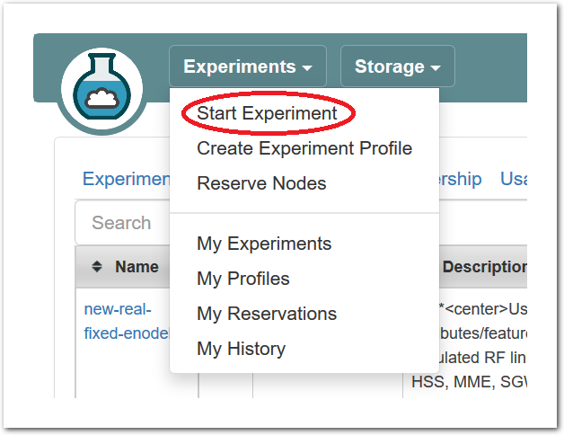 After logging in, you are taken to your main status dashboard. Select “Start Experiment” from the “Experiments” menu.
 - Select a profile
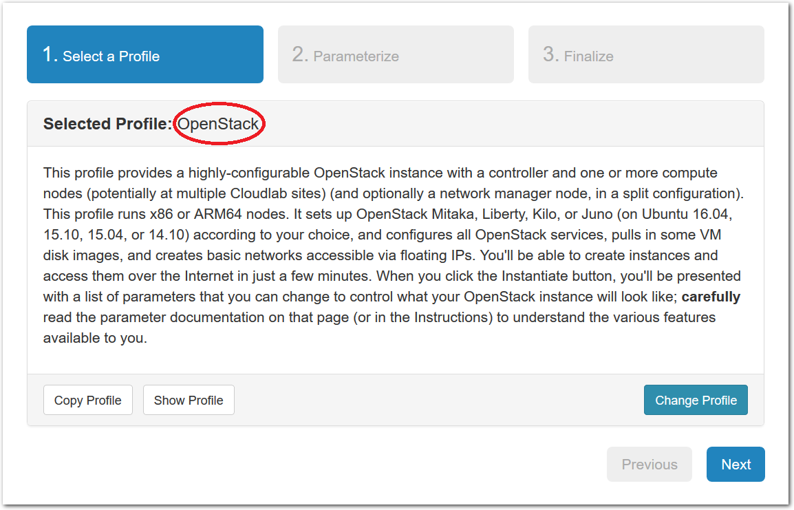 The “Start an Experiment” page is where you will select a profile to instantiate. We will use the k8s profile. You can select that profile by using this link or clicking the “Change Profile” button, and searching for “k8s“ in the list on the left. There may be multiple profiles with “k8s” in the name, so make sure you are using the one listed as a “System” profile as shown in the screenshot below.
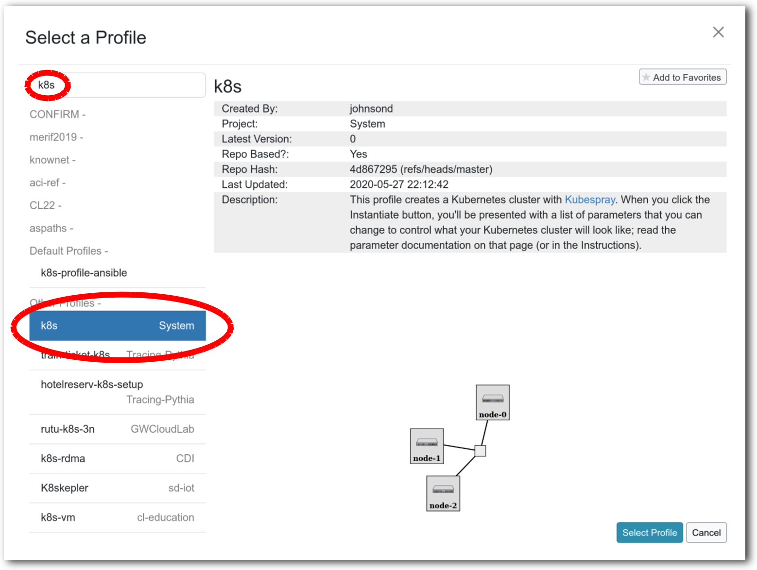
CloudLab allows its users to share their profiles, including by making them public. This is why there may be multiple “k8s” profiles listed. Profiles listed as “System” are created and supported by the CloudLab staff.
Once you have the correct profile selected, click “Next”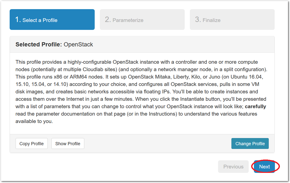
- Set parametersProfiles in CloudLab can have parameters that affect how they are configured; for example, this profile has parameters that let you control the size of your cluster and adjust many Kubernetes options.Note: If you are at an in-person tutorial, the presenter may ask you to set parameters such as the node type or number of nodes.Otherwise, you can leave all parameters at their defaults and just click “next”.

- Select a clusterCloudLab has multiple clusters available to it. Some profiles can run on any cluster, some can only run on specific ones due to specific hardware constraints, etc.
You may optionally give your experiment a name—
this can be useful if you have many experiments running at once. Note: If you are at an in-person tutorial, the instructor will tell you which cluster to select. Additionally, if you selected a node type in the parameterize step, you may not see a cluster selector - this is because most node types exist at only one cluster. Otherwise, you may select any cluster.You may see “calendar” icons in the cluster list - this indicates that you, or your project, have a reservation on that cluster. Usually, this means that’s the cluster you’ll want to select.
The dropdown menu for the clusters shows you both the health (outer ring) and available resources (inner dot) of each cluster. The “Check Cluster Status” link opens a page (in a new tab) showing the current utilization of all CloudLab clusters.
Click “Next”.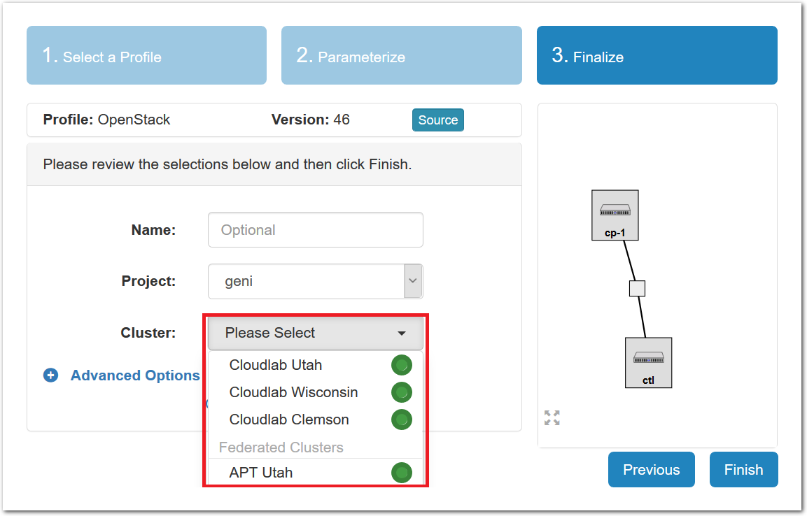
- Click Finish!CloudLab has the ability to schedule experiments to run in the future. For this tutorial, we’ll just run it right now. When you click the “finish” button, CloudLab will start provisioning the resources that you requested on the cluster that you selected.

- CloudLab instantiates your profileCloudLab will take a few minutes to bring up your copy of Kubernetes, as many things happen at this stage, including selecting suitable hardware, loading disk images on local storage, booting bare-metal machines, re-configuring the network topology, etc. While this is happening, you will see this status page:
 As soon as a set of resources have been assigned to you, you will see details about them at the bottom of the page (though you will not be able to log in until they have gone through the process of imaging and booting.) While you are waiting for your resources to become available, you may want to have a look at the CloudLab user manual, or use the “Logs” button to watch the logs of the resources being provisioned and booting.
 - Your cluster boots and runs startup scriptsWhen the web interface reports the state as “Booted”, this means that provisioning (such as disk imaging, network setup, and booting) is finished. This profile has startup scripts that run after the nodes boot - these may still be running when you first look at the status page. You can get details about which nodes have finished and which are still running under the “List View” tab.
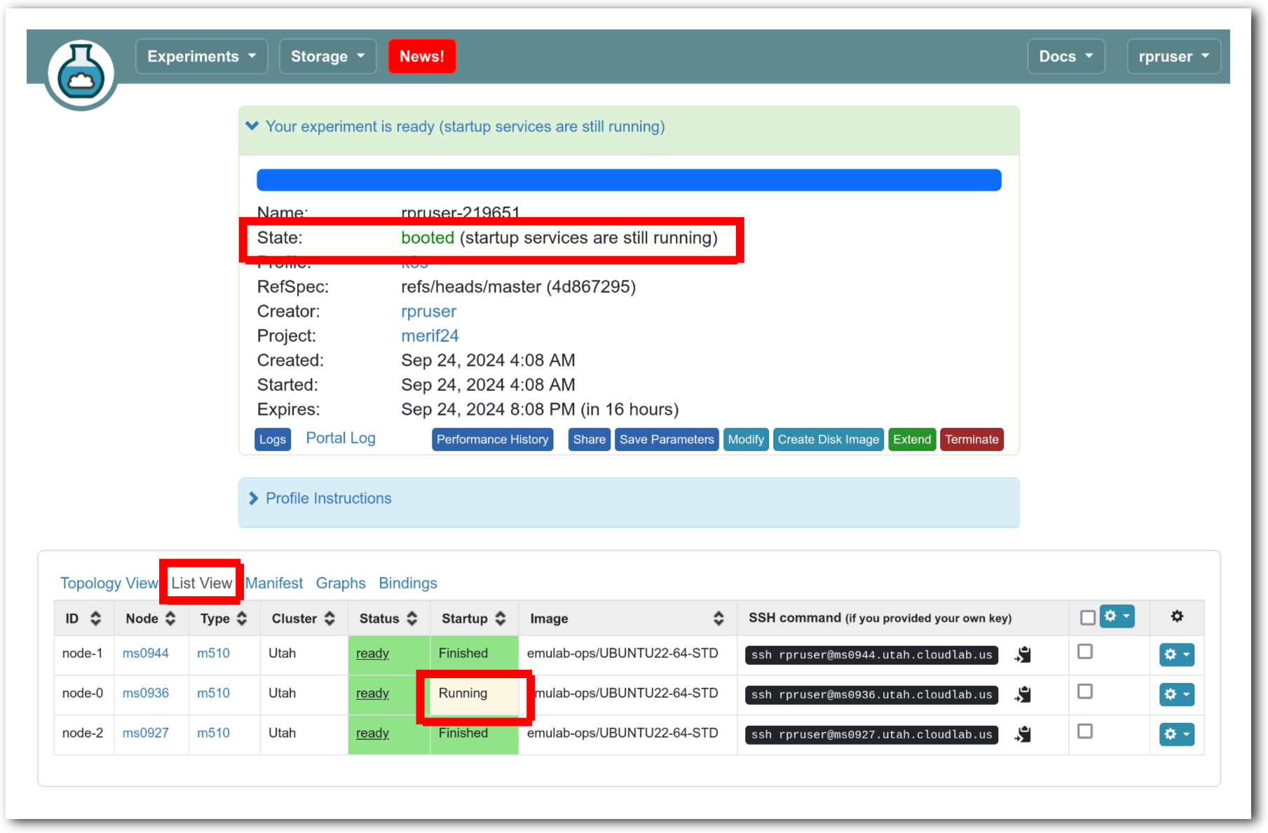
- Your cluster is ready!When the web interface reports the state as “Ready”, startup scripts are done running, and you can proceed to the next section. For now, don’t attempt to log in to Kubernetes we will explore the CloudLab experiment first.
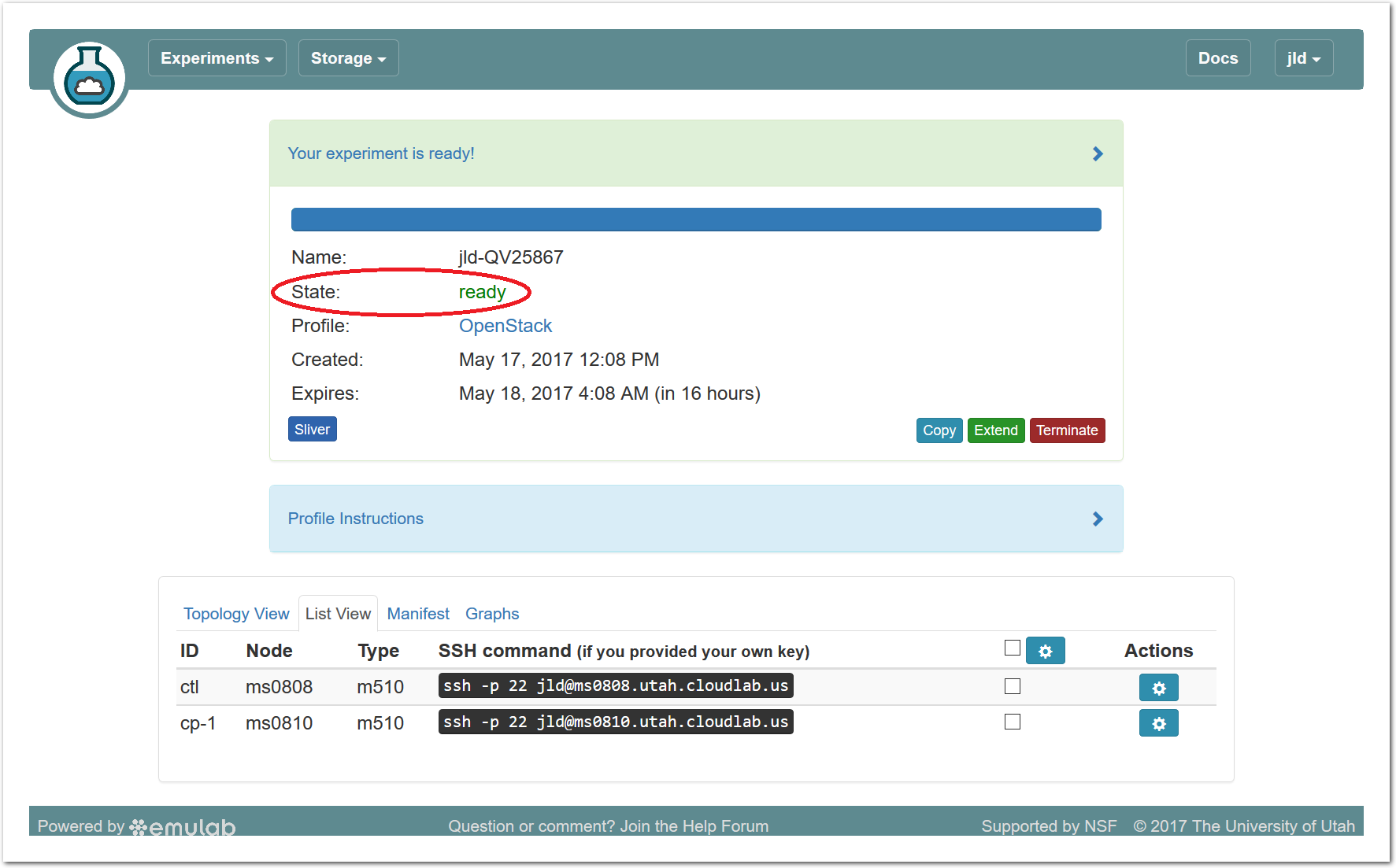
14.5 Exploring Your Experiment
Now that your experiment is ready, take a few minutes to look at various parts of the CloudLab status page to help you understand what resources you’ve got and what you can do with them.
14.5.1 Experiment Status
The panel at the top of the page shows the status of your experiment—
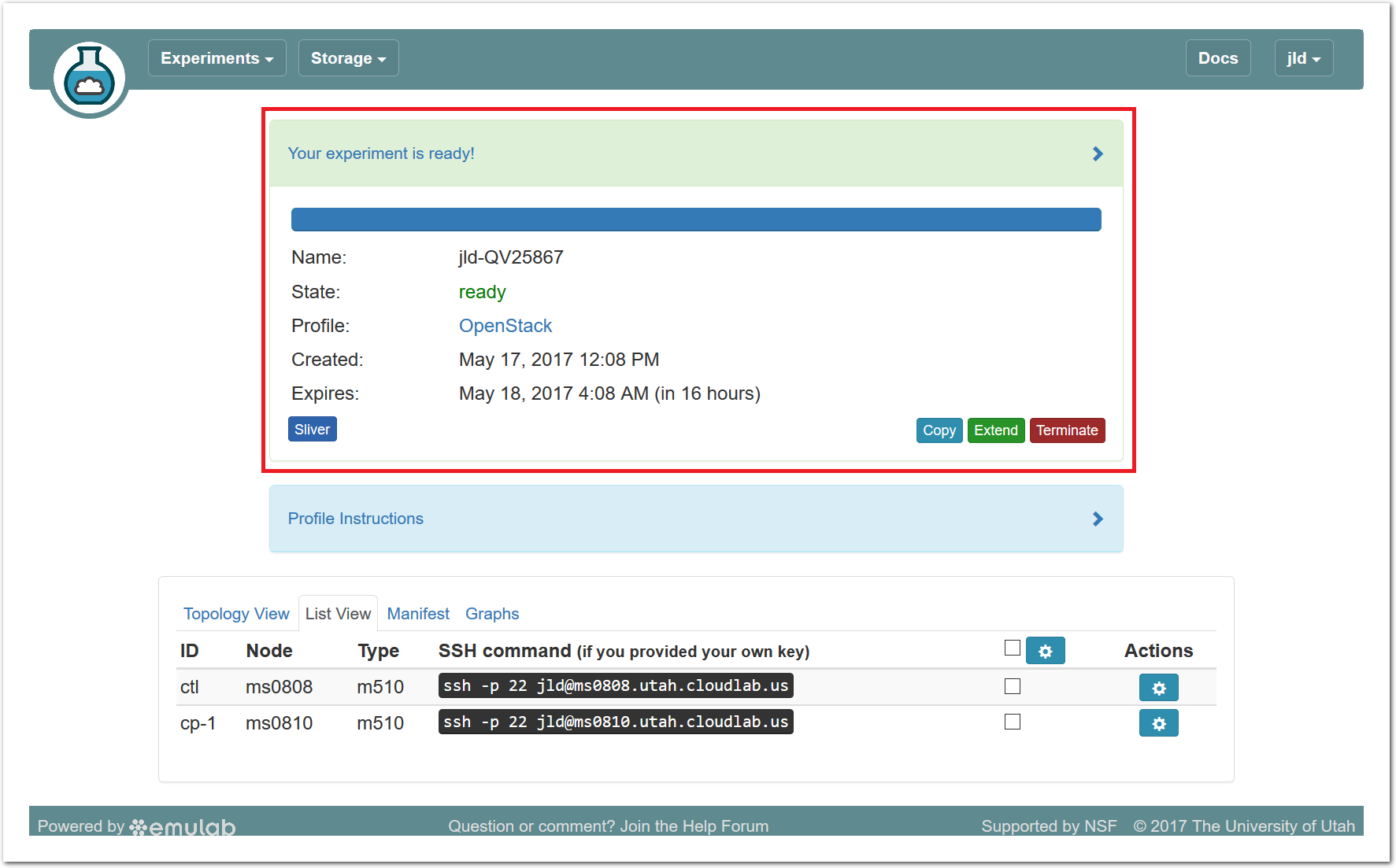
Note that the default lifetime for experiments on CloudLab is less than a day; after this time, the resources will be reclaimed and their disk contents will be lost. If you need to use them for longer, you can use the “Extend” button and provide a description of why they are needed. Longer extensions require higher levels of approval from CloudLab staff. You might also consider creating a profile of your own if you might need to run a customized environment multiple times or want to share it with others.
You can click the title of the panel to expand or collapse it.
14.5.2 Profile Instructions
Profiles may contain written instructions for their use. Clicking on the title
of the “Profile Instructions” panel will expand (or collapse) it; in this
case, the instructions provide a link to the dashboard of
Kubernetes, and give you passwords to use to log in. (Don’t log into Kubernetes
yet—
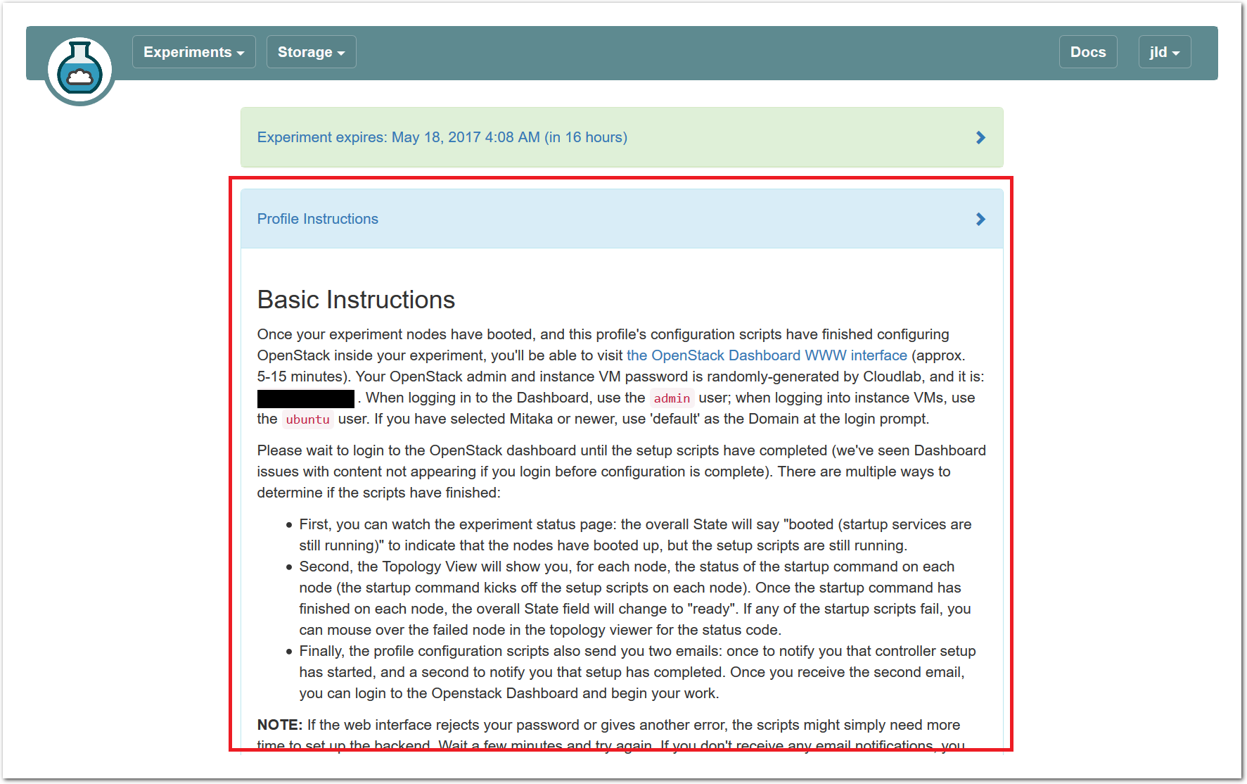
14.5.3 Topology View
At the bottom of the page, you can see the topology of your experiment. This profile has three nodes connected by a LAN, which is represented by a gray box in the middle of the topology. The names given for each node are the names assigned as part of the profile; this way, every time you instantiate a profile, you can refer to the nodes using the same names, regardless of which physical hardware was assigned to them. The green boxes around each node indicate that they are up; click the “Refresh Status” button to initiate a fresh check.
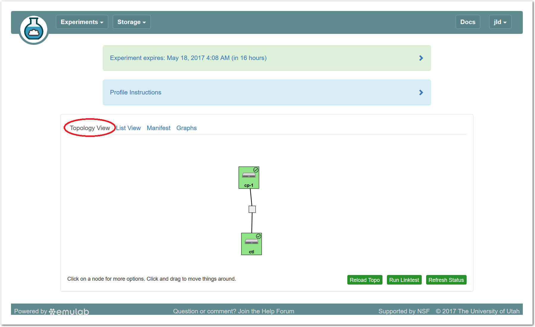
If an experiment has “startup services” (programs that run at the beginning of the experiment to set it up), their status is indicated by a small icon in the upper right corner of the node. You can mouse over this icon to see a description of the current status. In this profile, the startup services on the compute node(s) typically complete quickly, but the control node may take much longer.
It is important to note that every node in CloudLab has at least two network interfaces: one “control network” that carries public IP connectivity, and one “experiment network” that is isolated from the Internet and all other experiments. It is the experiment net that is shown in this topology view. You will use the control network to ssh into your nodes, interact with their web interfaces, etc. This separation gives you more freedom and control in the private experiment network, and sets up a clean environment for repeatable research.
14.5.4 List View
The list view tab shows similar information to the topology view, but in a different format. It shows the identities of the nodes you have been assigned, and the full ssh command lines to connect to them. In some browsers (those that support the ssh:// URL scheme), you can click on the SSH commands to automatically open a new session. On others, you may need to cut and paste this command into a terminal window. Note that only public-key authentication is supported, and you must have set up an ssh keypair on your account before starting the experiment in order for authentication to work.

14.5.5 Manifest View
The third default tab shows a manifest detailing the hardware that has been assigned to you. This is the “request” RSpec that is used to define the profile, annotated with details of the hardware that was chosen to instantiate your request. This information is available on the nodes themselves using the geni-get command, enabling you to do rich scripting that is fully aware of both the requested topology and assigned resources.
Most of the information displayed on the CloudLab status page comes directly from this manifest; it is parsed and laid out in-browser.

14.5.6 Graphs View
The final default tab shows a page of CPU load and network traffic graphs for the nodes in your experiment. On a freshly-created experiment, it may take several minutes for the first data to appear. After clicking on the “Graphs” tab the first time, a small reload icon will appear on the tab, which you can click to refresh the data and regenerate the graphs. For instance, here is the load average graph for an experiment running for over 6 hours. Scroll past this screenshot to see the control and experiment network traffic graphs. In your experiment, you’ll want to wait 20-30 minutes before expecting to see anything interesting.
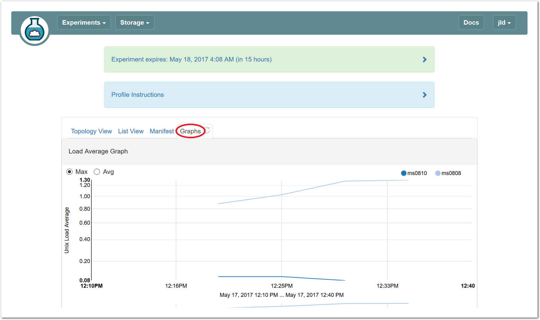
Here are the control network and experiment network packet graphs at the same time. The spikes at the beginning are produced by the initial profile setup and, as well as the simple tasks you’ll perform later in this profile.
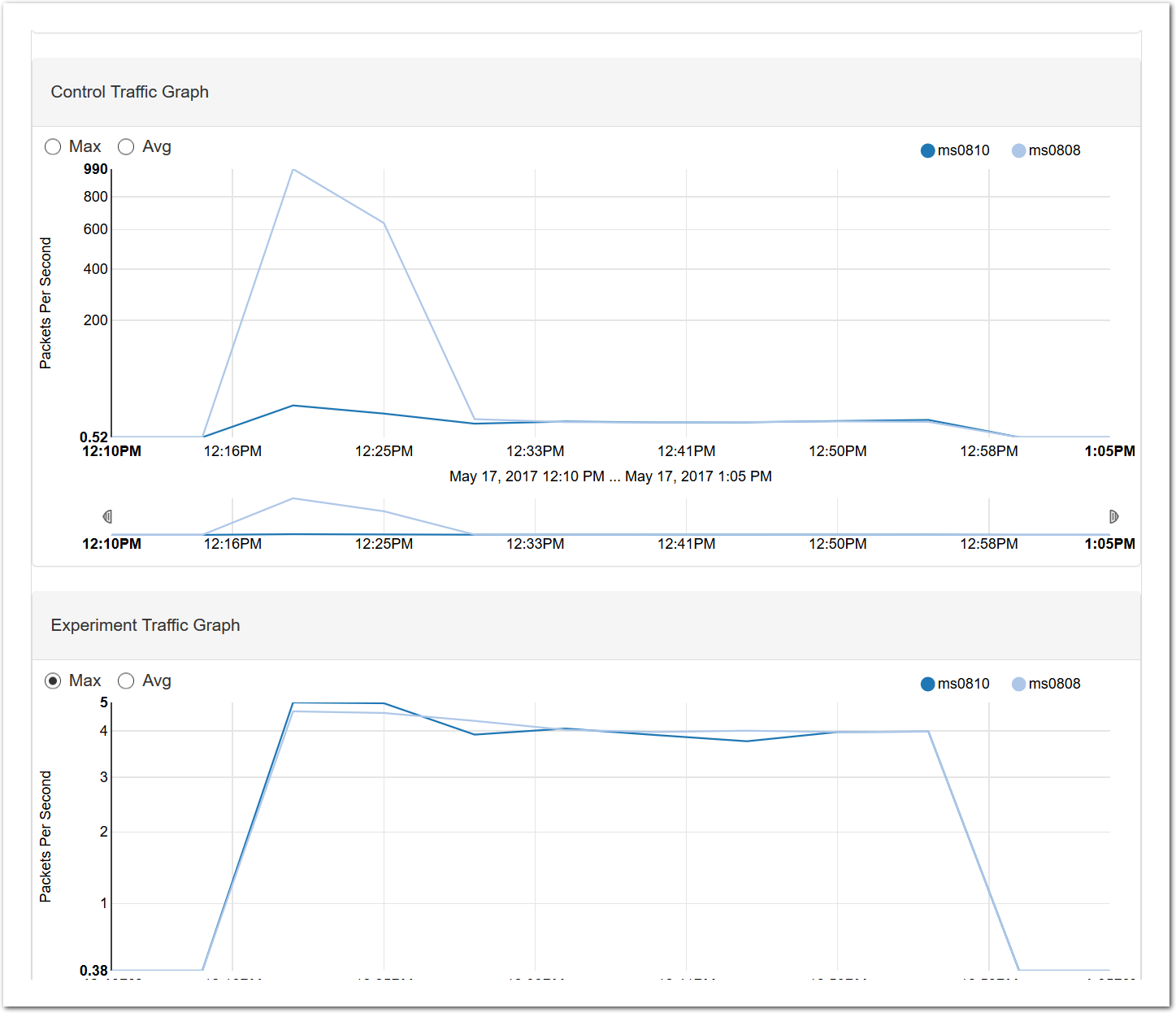
14.5.7 Actions
In both the topology and list views, you have access to several actions that you may take on individual nodes. In the topology view, click on the node to access this menu; in the list view, it is accessed through the icon in the “Actions” column. Available actions include rebooting (power cycling) a node, and re-loading it with a fresh copy of its disk image (destroying all data on the node). While nodes are in the process of rebooting or re-imaging, they will turn yellow in the topology view. When they have completed, they will become green again. The shell and console actions are described in more detail below.
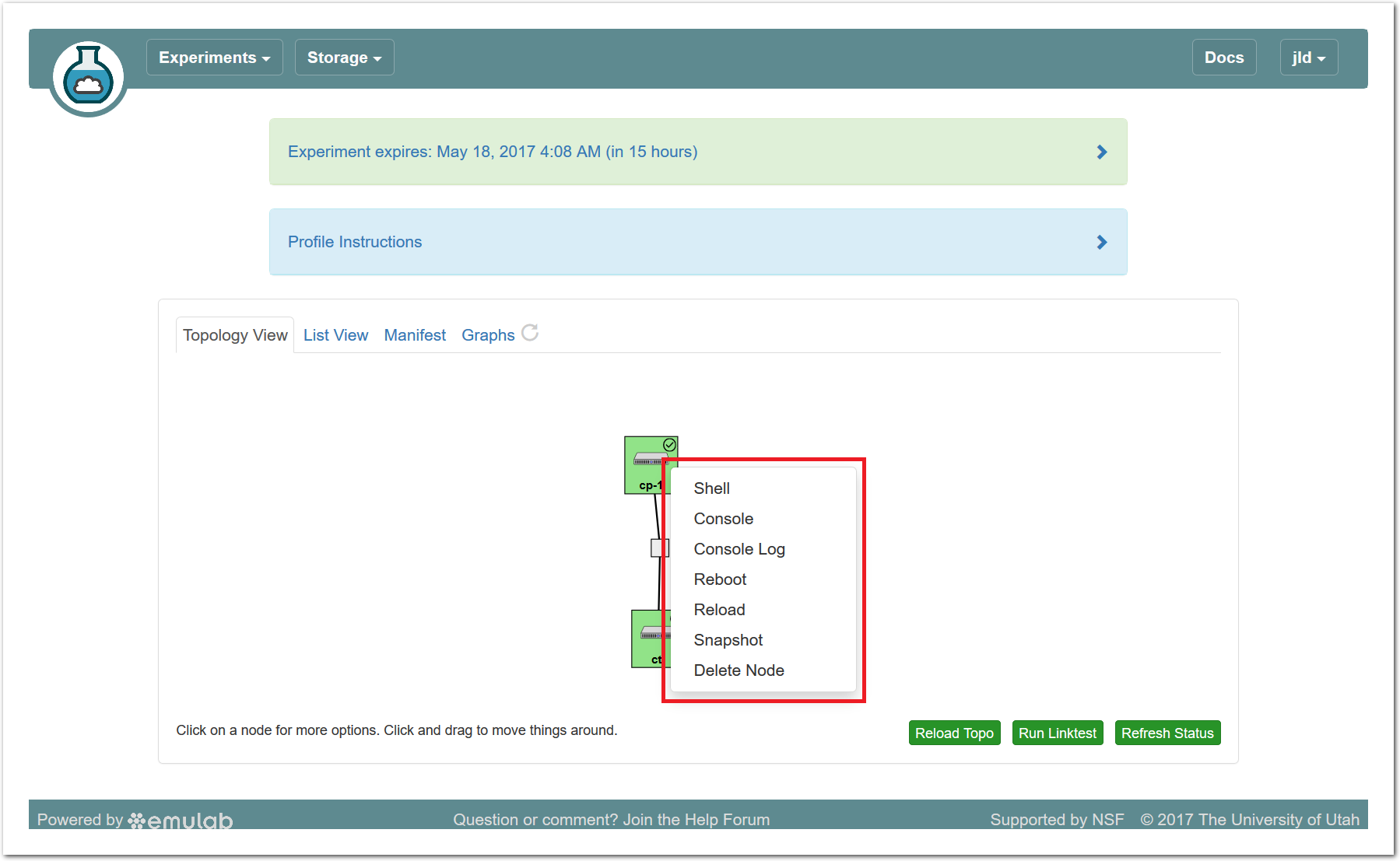
14.5.8 Web-based Shell
CloudLab provides a browser-based shell for logging into your nodes, which is accessed through the action menu described above. While this shell is functional, it is most suited to light, quick tasks; if you are going to do serious work, on your nodes, we recommend using a standard terminal and ssh program.
This shell can be used even if you did not establish an ssh keypair with your account.
Two things of note:
Your browser may require you to click in the shell window before it gets focus.
Depending on your operating system and browser, cutting and pasting into the window may not work. If keyboard-based pasting does not work, try right-clicking to paste.
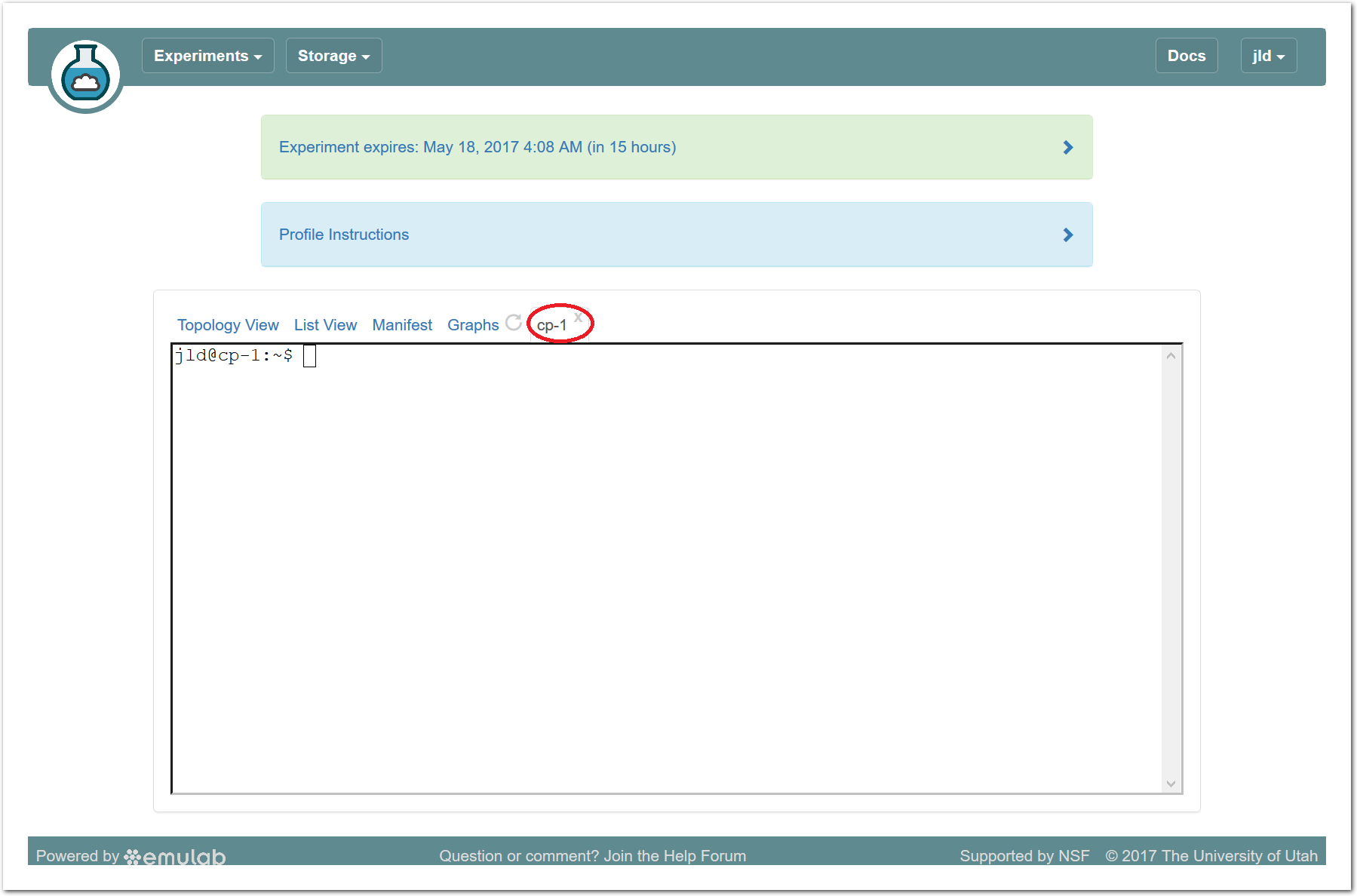
14.5.9 Serial Console
CloudLab provides serial console access for all nodes, which can be used in the event that normal IP or ssh access gets intentionally or unintentionally broken. Like the browser-based shell, it is launched through the access menu, and the same caveats listed above apply as well. In addition:
If you look at the console for a node that is already booted, the console may be blank due to a lack of activity; press enter several times to get a fresh login prompt.
If you need to log in, do so as root; your normal user account does not allow password login. There is a link above the console window that reveals the randomly-generated root password for your node. Note that this password changes frequently for security reasons.
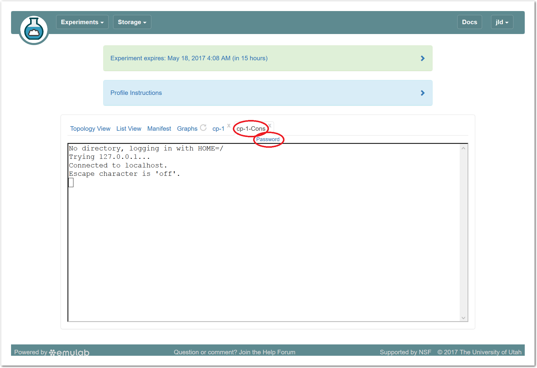
14.6 Exploring Kubernetes
Now that you have your own copy of Kubernetes running, you can use it just like you would any other Kubernetes cluster, with the important property that you have full root access to every machine in the cluster and can modify them however you’d like.
14.6.1 Kubernetes Dashboard
Following the directions under the “Kubernetes credentials and dashboard access” portion of the profile instructions, click the link for the authentication token, which will be a URL leading to one of the CloudLab nodes in your experiment. You will be asked for a username (“admin”) and password (found in the profile instructions).
The admin password is randomly generated for each experiment.
Copy the entire contents of the file you are presented with, and go back to the profile instructions. Near the top of the “Kubernetes credentials ...” section, you will find a link to your dashboard, again hosted on one of the nodes in your experiment. Click the link (you may have to tell your browser to accept the self-signed TLS certificate) and you’ll see the Kubernetes dashboard login page.
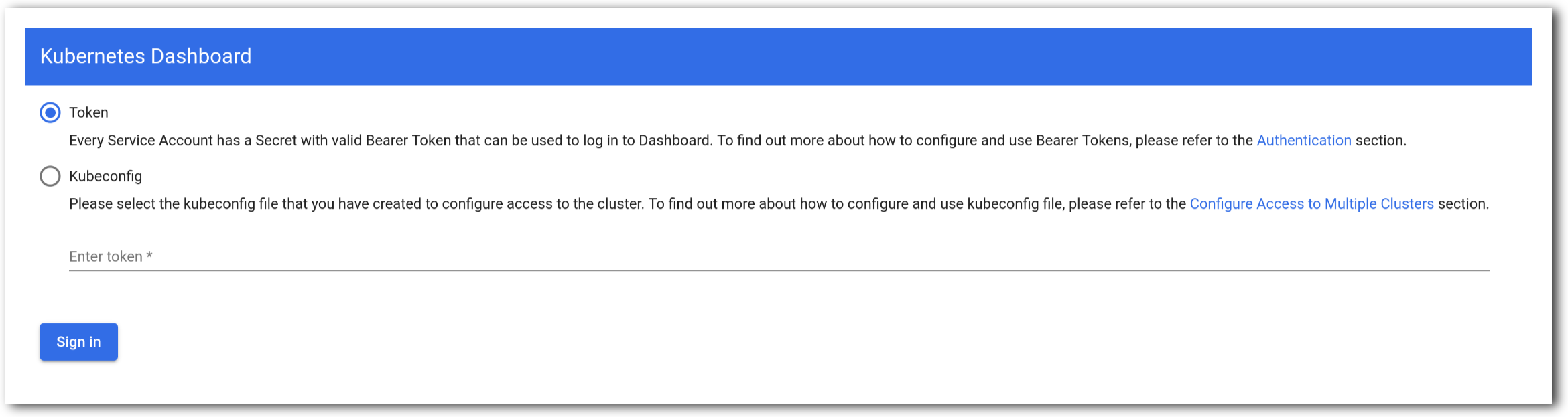
Make sure that “token” is selected and paste in the token you copied. Once logged in, you’ll be able to see the status of your cluster, including the current workload (there won’t be much running), the set of nodes, and much more.
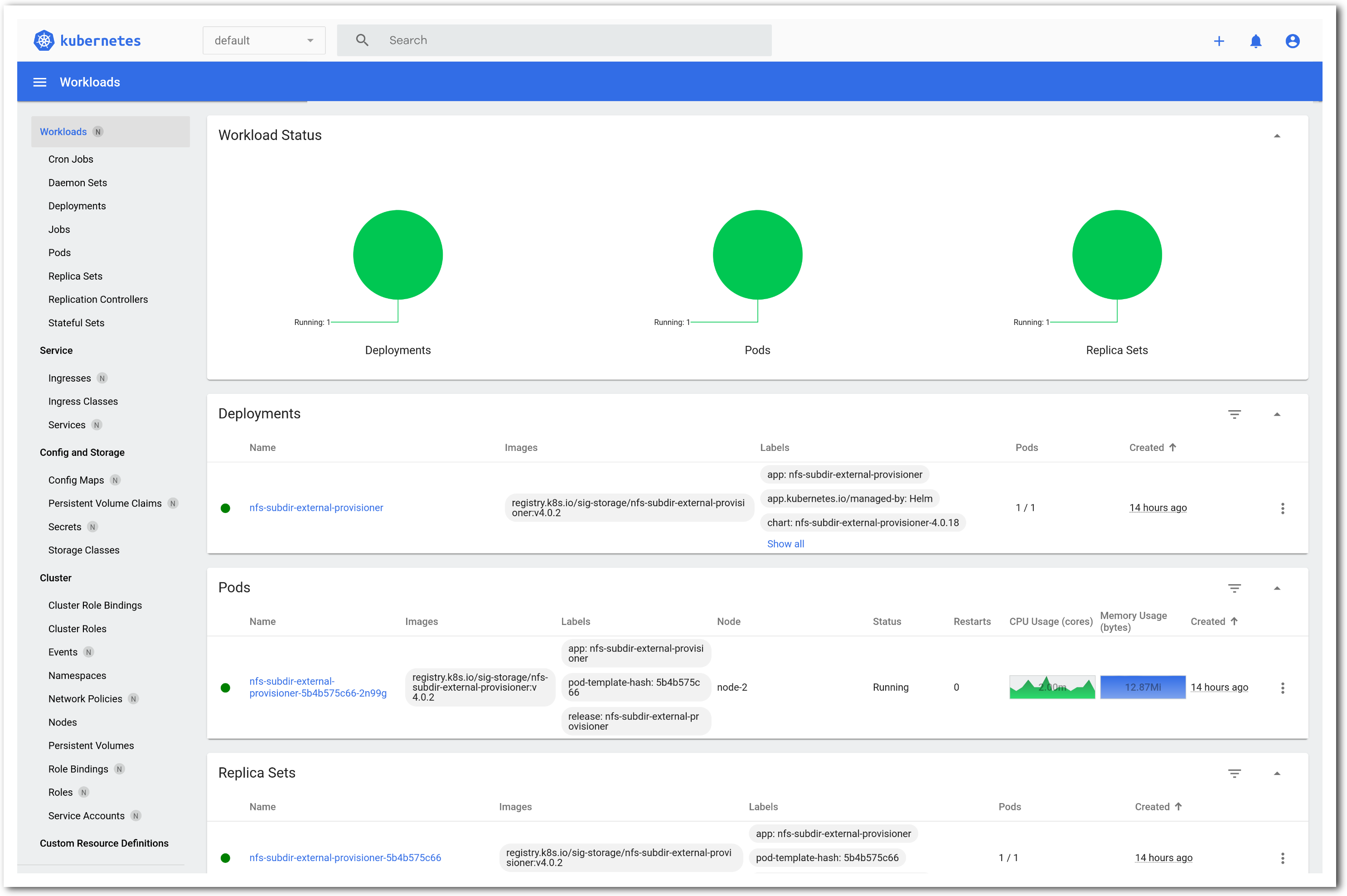
14.6.2 Kubernetes Dashboard
If you want to start jobs in Kubernetes, you’ll need to use the command line. Start a shell on “node-0” using the instructions above. You can run kubectl on these nodes; our profile also installs helm.
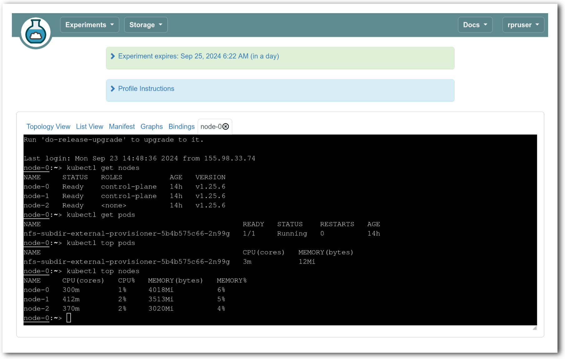
14.7 Terminating the Experiment
Resources that you hold in CloudLab are real, physical machines and are therefore limited and in high demand. When you are done, you should release them for use by other experimenters. Do this via the “Terminate” button on the CloudLab experiment status page.
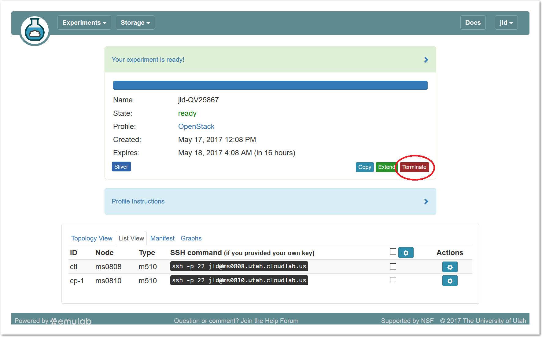
Note: When you terminate an experiment, all data on the nodes is lost, so make sure to copy off any data you may need before terminating.
If you were doing a real experiment, you might need to hold onto the nodes for longer than the default expiration time. You would request more time by using the “Extend” button the on the status page. You would need to provide a written justification for holding onto your resources for a longer period of time.
14.8 Taking Next Steps
Now that you’ve got a feel for for what CloudLab can do, there are several things you might try next:
Create a new project to continue working on CloudLab past this tutorial
Try out some profiles other than k8s (use the “Change Profile” button on the “Start Experiment” page)
Read more about the basic concepts in CloudLab
Try out different hardware
Learn how to make your own profiles
15 CloudLab OpenStack Tutorial
This tutorial will walk you through the process of creating a small cloud on CloudLab using OpenStack. Your copy of OpenStack will run on bare-metal machines that are dedicated for your use for the duration of your experiment. You will have complete administrative access to these machines, meaning that you have full ability to customize and/or configure your installation of OpenStack.
15.1 Objectives
In the process of taking this tutorial, you will learn to:
Log in to CloudLab
Create your own cloud by using a pre-defined profile
Access resources in a cloud that you create
Use administrative access to customize your cloud
Clean up your cloud when finished
Learn where to get more information
15.2 Prerequisites
This tutorial assumes that:
- You have an existing account on either:
CloudLab (Instructions for getting an account can be found here.)
The GENI portal. (Instructions for getting an account can be found here.)
16.4 Logging In
If you have signed up for an account at the CloudLab website, simply open https://www.cloudlab.us/ in your browser, click the “Log In” button, enter your username and password.
15.4 Building Your Own OpenStack Cloud
Once you have logged in to CloudLab, you will “instantiate” a “profile” to create an experiment. (An experiment in CloudLab is similar to a “slice” in GENI.) Profiles are CloudLab’s way of packaging up configurations and experiments so that they can be shared with others. Each experiment is separate: the experiment that you create for this tutorial will be an instance of a profile provided by the facility, but running on resources that are dedicated to you, which you have complete control over. This profile uses local disk space on the nodes, so anything you store there will be lost when the experiment terminates.
The OpenStack cloud we will build in this tutorial is very small, but CloudLab has additional hardware that can be used for larger-scale experiments.
For this tutorial, we will use a basic profile that brings up a small OpenStack cloud. The CloudLab staff have built this profile by capturing disk images of a partially-completed OpenStack installation and scripting the remainder of the install (customizing it for the specific machines that will get allocated, the user that created it, etc.) See this manual’s section on profiles for more information about how they work.
- Start ExperimentAfter logging in, you are taken to your main status dashboard. Select “Start Experiment” from the “Experiments” menu.
- Select a profile
 The “Start an Experiment” page is where you will select a profile to instantiate. We will use the OpenStack profile; if it is not selected, follow this link or click the “Change Profile” button, and select “OpenStack” from the list on the left.Once you have the correct profile selected, click “Next”
- Set parametersProfiles in CloudLab can have parameters that affect how they are configured; for example, this profile has parameters that allow you to set the size of your cloud, spread it across multiple clusters, and turn on and off many OpenStack options.For this tutorial, we will leave all parameters at their defaults and just click “next”.
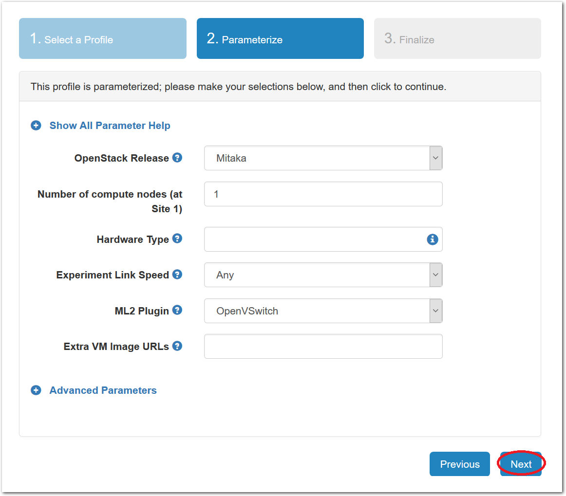
- Select a clusterCloudLab has multiple clusters available to it. Some profiles can run on any cluster, some can only run on specific ones due to specific hardware constraints, etc.Note: If you are at an in-person tutorial, the instructor will tell you which cluster to select. Otherwise, you may select any cluster.
The dropdown menu for the clusters shows you both the health (outer ring) and available resources (inner dot) of each cluster. The “Check Cluster Status” link opens a page (in a new tab) showing the current utilization of all CloudLab clusters.

- Click Finish!When you click the “finish” button, CloudLab will start provisioning the resources that you requested on the cluster that you selected.
You may optionally give your experiment a name—
this can be useful if you have many experiments running at once. 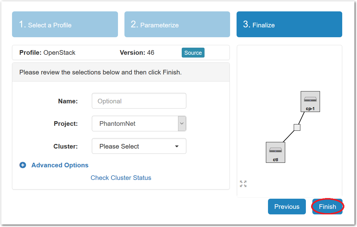
- CloudLab instantiates your profileCloudLab will take a few minutes to bring up your copy of OpenStack, as many things happen at this stage, including selecting suitable hardware, loading disk images on local storage, booting bare-metal machines, re-configuring the network topology, etc. While this is happening, you will see this status page:
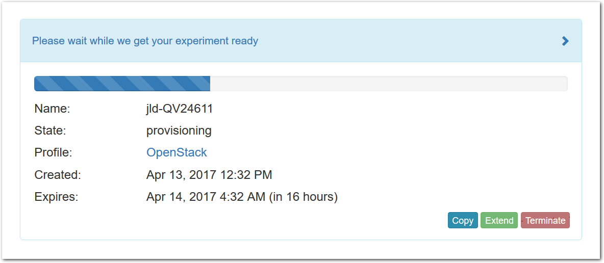
Provisioning is done using the GENI APIs; it is possible for advanced users to bypass the CloudLab portal and call these provisioning APIs from their own code. A good way to do this is to use the geni-lib library for Python.
As soon as a set of resources have been assigned to you, you will see details about them at the bottom of the page (though you will not be able to log in until they have gone through the process of imaging and booting.) While you are waiting for your resources to become available, you may want to have a look at the CloudLab user manual, or use the “Sliver” button to watch the logs of the resources (“slivers”) being provisioned and booting. - Your cloud is ready!When the web interface reports the state as “Booted”, your cloud is provisioned, and you can proceed to the next section.Important: A “Booted” status indicates that resources are provisioned and booted; this particular profile runs scripts to complete the OpenStack setup, and it will be a few more minutes before OpenStack is fully ready to log in and create virtual machine instances. You will be able to tell that this has finished when the status changes from “Booted” to “Ready”. For now, don’t attempt to log in to OpenStack, we will explore the CloudLab experiment first.
15.5 Exploring Your Experiment
Now that your experiment is ready, take a few minutes to look at various parts of the CloudLab status page to help you understand what resources you’ve got and what you can do with them.
15.5.1 Experiment Status
The panel at the top of the page shows the status of your experiment—

Note that the default lifetime for experiments on CloudLab is less than a day; after this time, the resources will be reclaimed and their disk contents will be lost. If you need to use them for longer, you can use the “Extend” button and provide a description of why they are needed. Longer extensions require higher levels of approval from CloudLab staff. You might also consider creating a profile of your own if you might need to run a customized environment multiple times or want to share it with others.
You can click the title of the panel to expand or collapse it.
15.5.2 Profile Instructions
Profiles may contain written instructions for their use. Clicking on the title
of the “Profile Instructions” panel will expand (or collapse) it; in this
case, the instructions provide a link to the administrative interface of
OpenStack, and give you passwords to use to log in. (Don’t log into OpenStack
yet—
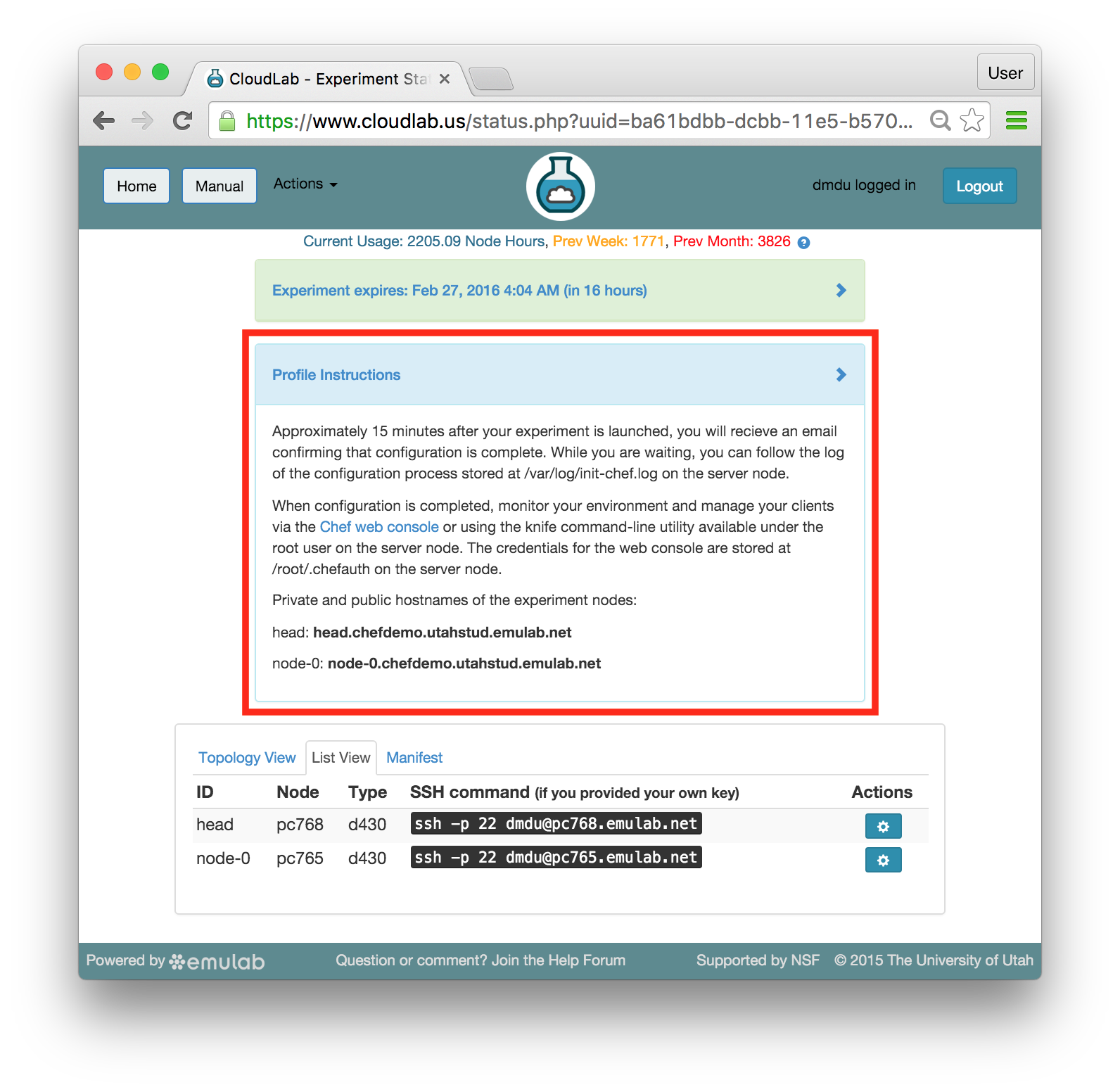
15.5.3 Topology View
At the bottom of the page, you can see the topology of your experiment. This profile has three nodes connected by a LAN, which is represented by a gray box in the middle of the topology. The names given for each node are the names assigned as part of the profile; this way, every time you instantiate a profile, you can refer to the nodes using the same names, regardless of which physical hardware was assigned to them. The green boxes around each node indicate that they are up; click the “Refresh Status” button to initiate a fresh check.
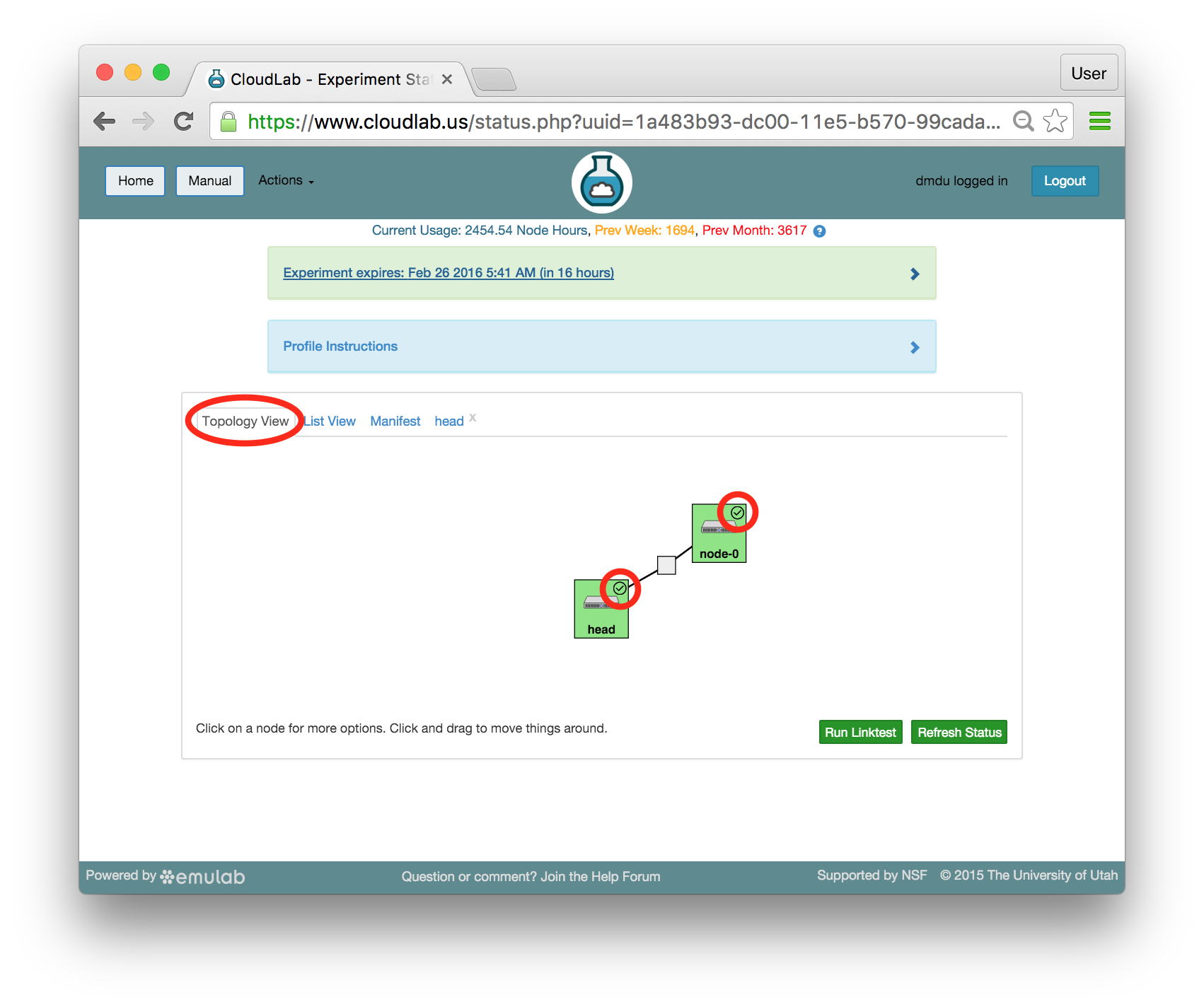
If an experiment has “startup services” (programs that run at the beginning of the experiment to set it up), their status is indicated by a small icon in the upper right corner of the node. You can mouse over this icon to see a description of the current status. In this profile, the startup services on the compute node(s) typically complete quickly, but the control node may take much longer.
It is important to note that every node in CloudLab has at least two network interfaces: one “control network” that carries public IP connectivity, and one “experiment network” that is isolated from the Internet and all other experiments. It is the experiment net that is shown in this topology view. You will use the control network to ssh into your nodes, interact with their web interfaces, etc. This separation gives you more freedom and control in the private experiment network, and sets up a clean environment for repeatable research.
15.5.4 List View
The list view tab shows similar information to the topology view, but in a different format. It shows the identities of the nodes you have been assigned, and the full ssh command lines to connect to them. In some browsers (those that support the ssh:// URL scheme), you can click on the SSH commands to automatically open a new session. On others, you may need to cut and paste this command into a terminal window. Note that only public-key authentication is supported, and you must have set up an ssh keypair on your account before starting the experiment in order for authentication to work.
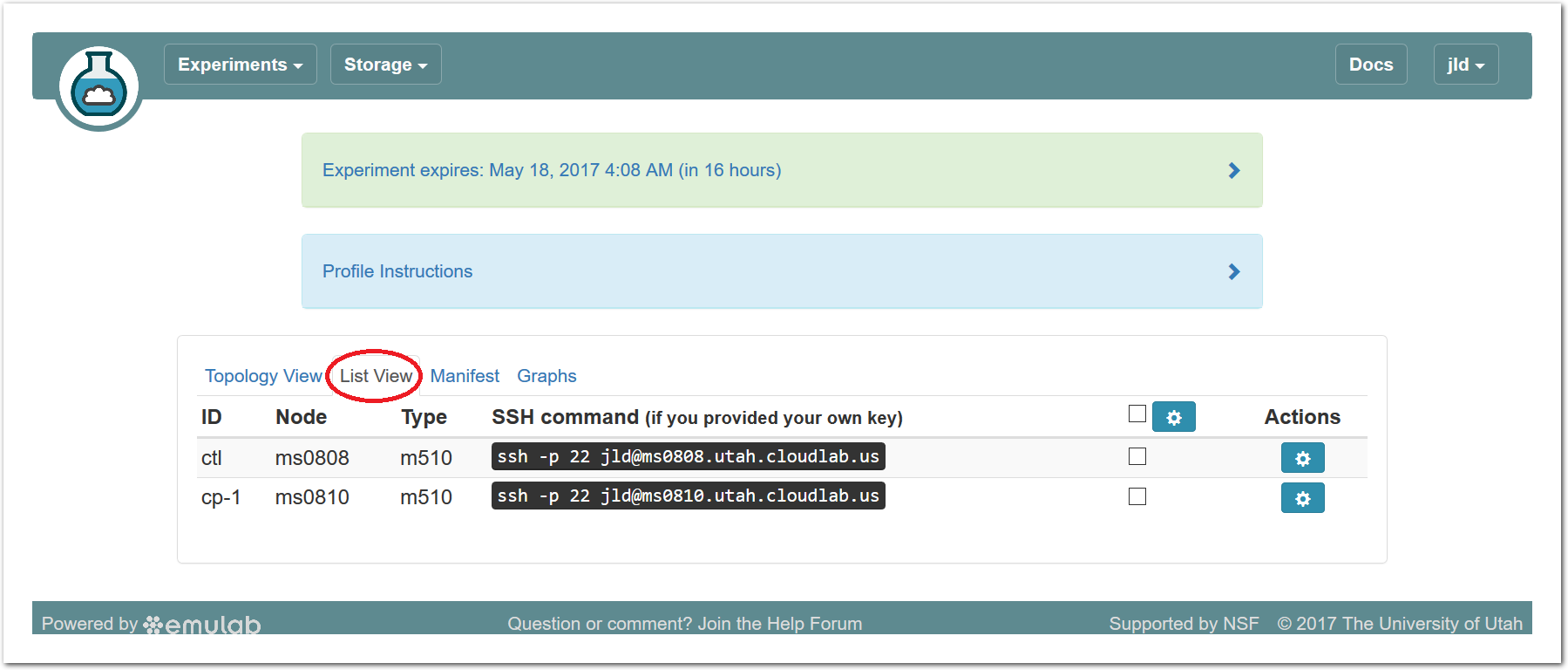
15.5.5 Manifest View
The third default tab shows a manifest detailing the hardware that has been assigned to you. This is the “request” RSpec that is used to define the profile, annotated with details of the hardware that was chosen to instantiate your request. This information is available on the nodes themselves using the geni-get command, enabling you to do rich scripting that is fully aware of both the requested topology and assigned resources.
Most of the information displayed on the CloudLab status page comes directly from this manifest; it is parsed and laid out in-browser.
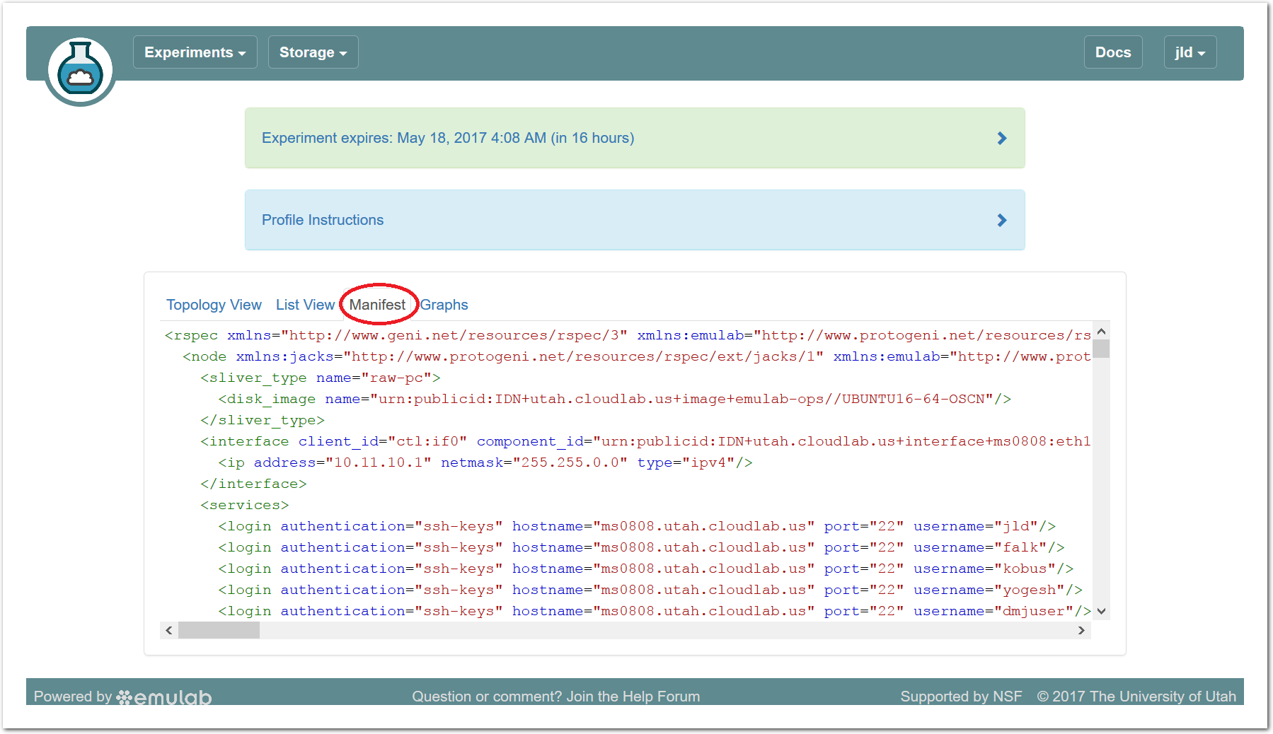
15.5.6 Graphs View
The final default tab shows a page of CPU load and network traffic graphs for the nodes in your experiment. On a freshly-created experiment, it may take several minutes for the first data to appear. After clicking on the “Graphs” tab the first time, a small reload icon will appear on the tab, which you can click to refresh the data and regenerate the graphs. For instance, here is the load average graph for an OpenStack experiment running this profile for over 6 hours. Scroll past this screenshot to see the control and experiment network traffic graphs. In your experiment, you’ll want to wait 20-30 minutes before expecting to see anything interesting.
Here are the control network and experiment network packet graphs at the same time. The spikes at the beginning are produced by OpenStack setup and configuration, as well as the simple OpenStack tasks you’ll perform later in this profile, like adding a VM.
15.5.7 Actions
In both the topology and list views, you have access to several actions that you may take on individual nodes. In the topology view, click on the node to access this menu; in the list view, it is accessed through the icon in the “Actions” column. Available actions include rebooting (power cycling) a node, and re-loading it with a fresh copy of its disk image (destroying all data on the node). While nodes are in the process of rebooting or re-imaging, they will turn yellow in the topology view. When they have completed, they will become green again. The shell and console actions are described in more detail below.
15.5.8 Web-based Shell
CloudLab provides a browser-based shell for logging into your nodes, which is accessed through the action menu described above. While this shell is functional, it is most suited to light, quick tasks; if you are going to do serious work, on your nodes, we recommend using a standard terminal and ssh program.
This shell can be used even if you did not establish an ssh keypair with your account.
Two things of note:
Your browser may require you to click in the shell window before it gets focus.
Depending on your operating system and browser, cutting and pasting into the window may not work. If keyboard-based pasting does not work, try right-clicking to paste.
15.5.9 Serial Console
CloudLab provides serial console access for all nodes, which can be used in the event that normal IP or ssh access gets intentionally or unintentionally broken. Like the browser-based shell, it is launched through the access menu, and the same caveats listed above apply as well. In addition:
If you look at the console for a node that is already booted, the console may be blank due to a lack of activity; press enter several times to get a fresh login prompt.
If you need to log in, do so as root; your normal user account does not allow password login. There is a link above the console window that reveals the randomly-generated root password for your node. Note that this password changes frequently for security reasons.
15.6 Bringing up Instances in OpenStack
Now that you have your own copy of OpenStack running, you can use it just like you would any other OpenStack cloud, with the important property that you have full root access to every machine in the cloud and can modify them however you’d like. In this part of the tutorial, we’ll go through the process of bringing up a new VM instance in your cloud.
We’ll be doing all of the work in this section using the Horizon web GUI for OpenStack, but you could also ssh into the machines directly and use the command line interfaces or other APIs as well.
- Check to see if OpenStack is ready to log inAs mentioned earlier, this profile runs several scripts to complete the installation of OpenStack. These scripts do things such as finalize package installation, customize the installation for the specific set of hardware assigned to your experiment, import cloud images, and bring up the hypervisors on the compute node(s).If exploring the CloudLab experiment took you more than ten minutes, these scripts are probably done. You can be sure by checking that all nodes have completed their startup scripts (indicated by a checkmark on the Topology view); when this happens, the experiment state will also change from “Booting” to “Ready”
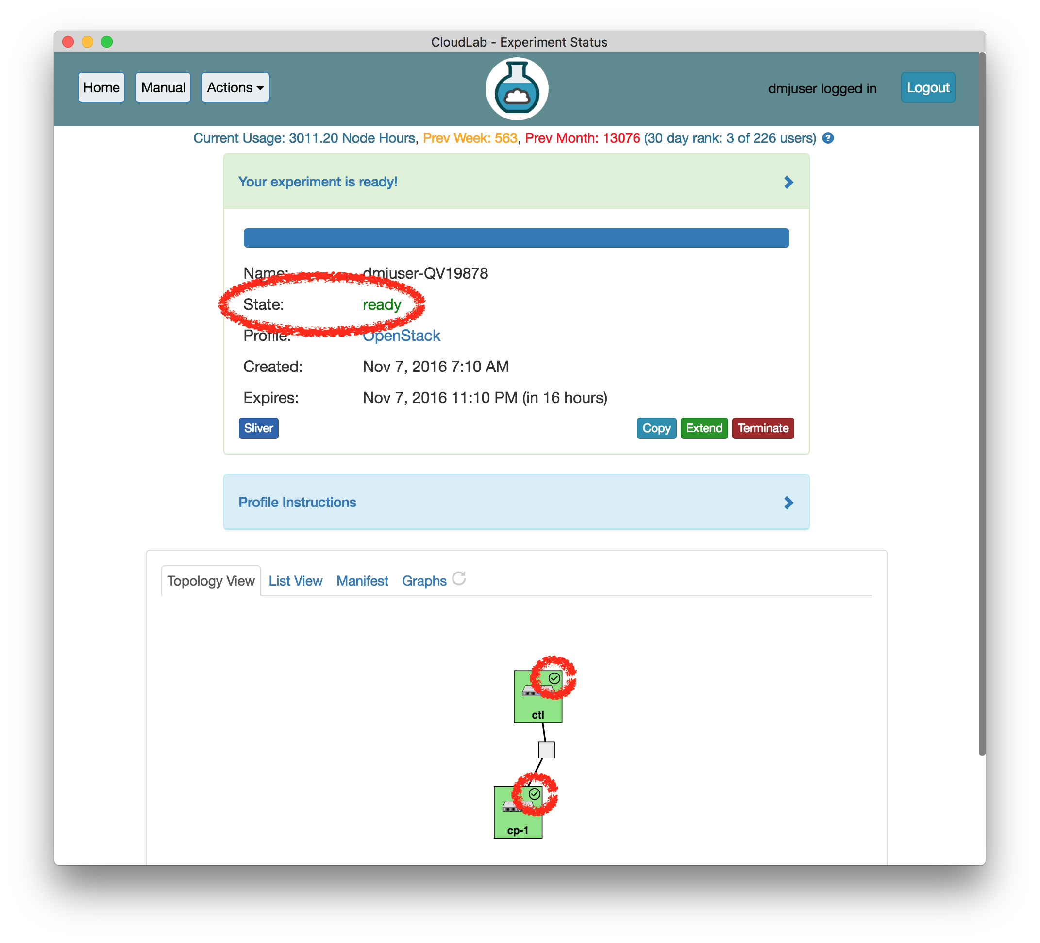 If you continue without verifying that the setup scripts are complete, be aware that you may see temporary errors from the OpenStack web interface. These errors, and the method for dealing with them, are generally noted in the text below.
 - Visit the OpenStack Horizon web interfaceOn the status page for your experiment, in the “Instructions” panel (click to expand it if it’s collapsed), you’ll find a link to the web interface running on the ctl node. Open this link (we recommend opening it in a new tab, since you will still need information from the CloudLab web interface).
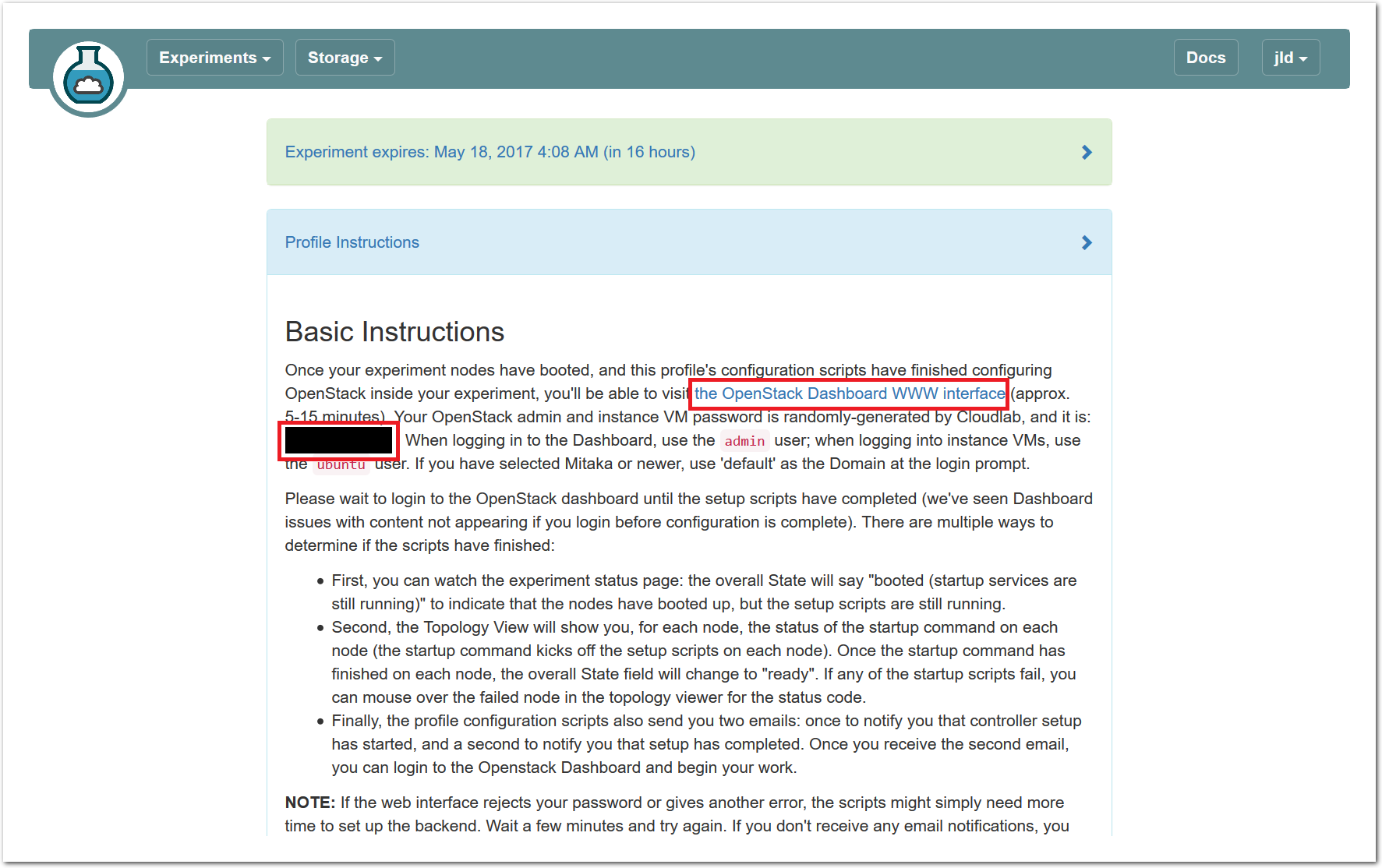
- Log in to the OpenStack web interfaceLog in using the username admin and the password shown in the instructions for the profile. Use the domain name default if prompted for a domain.
This profile generates a new (random) password for every experiment.
Important: if the web interface rejects your password, wait a few minutes and try again. If it gives you another type of error, you may need to wait a minute and reload the page to get login working properly.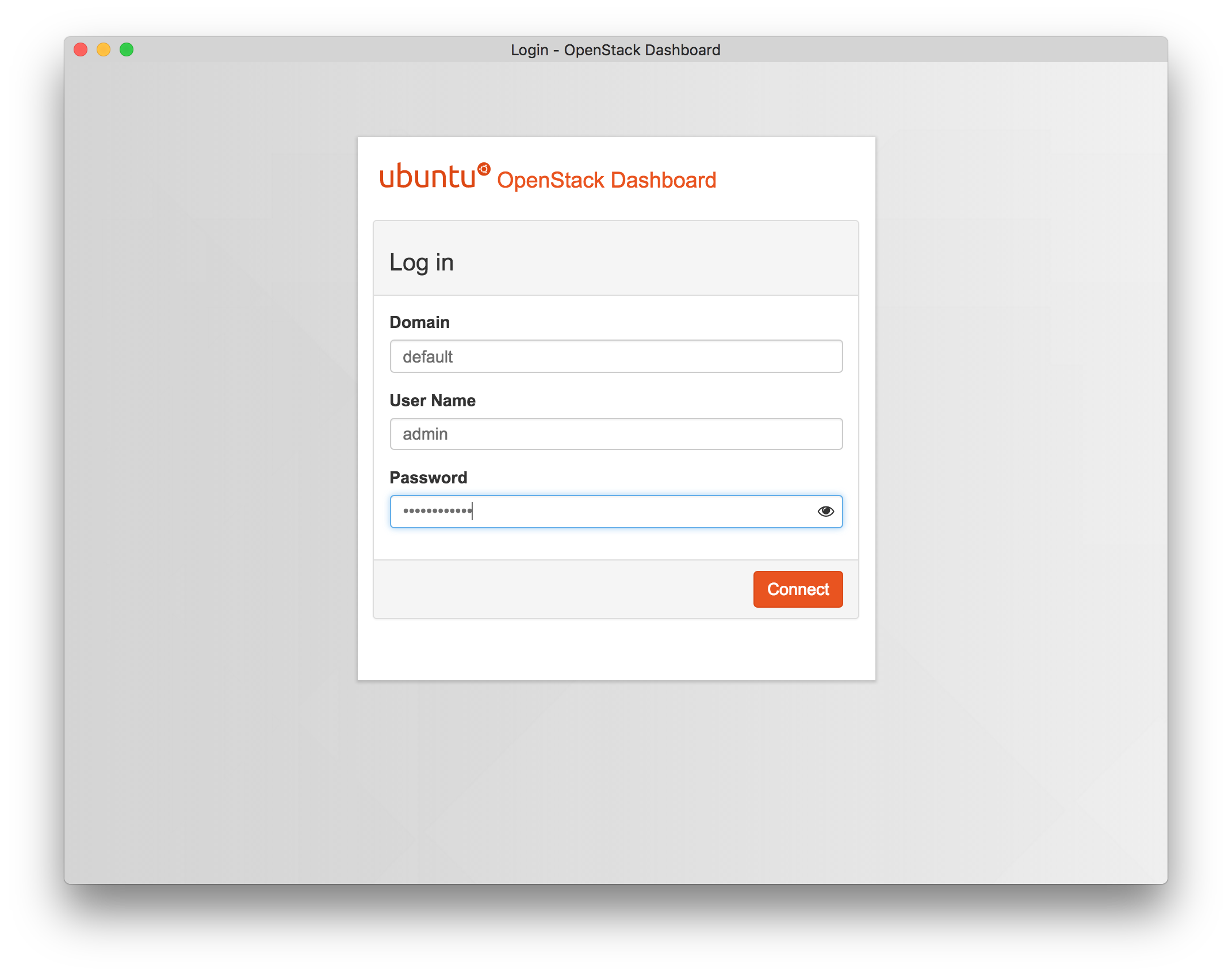
- Launch a new VM instanceClick the “Launch Instance” button on the “Instances” page of the web interface.
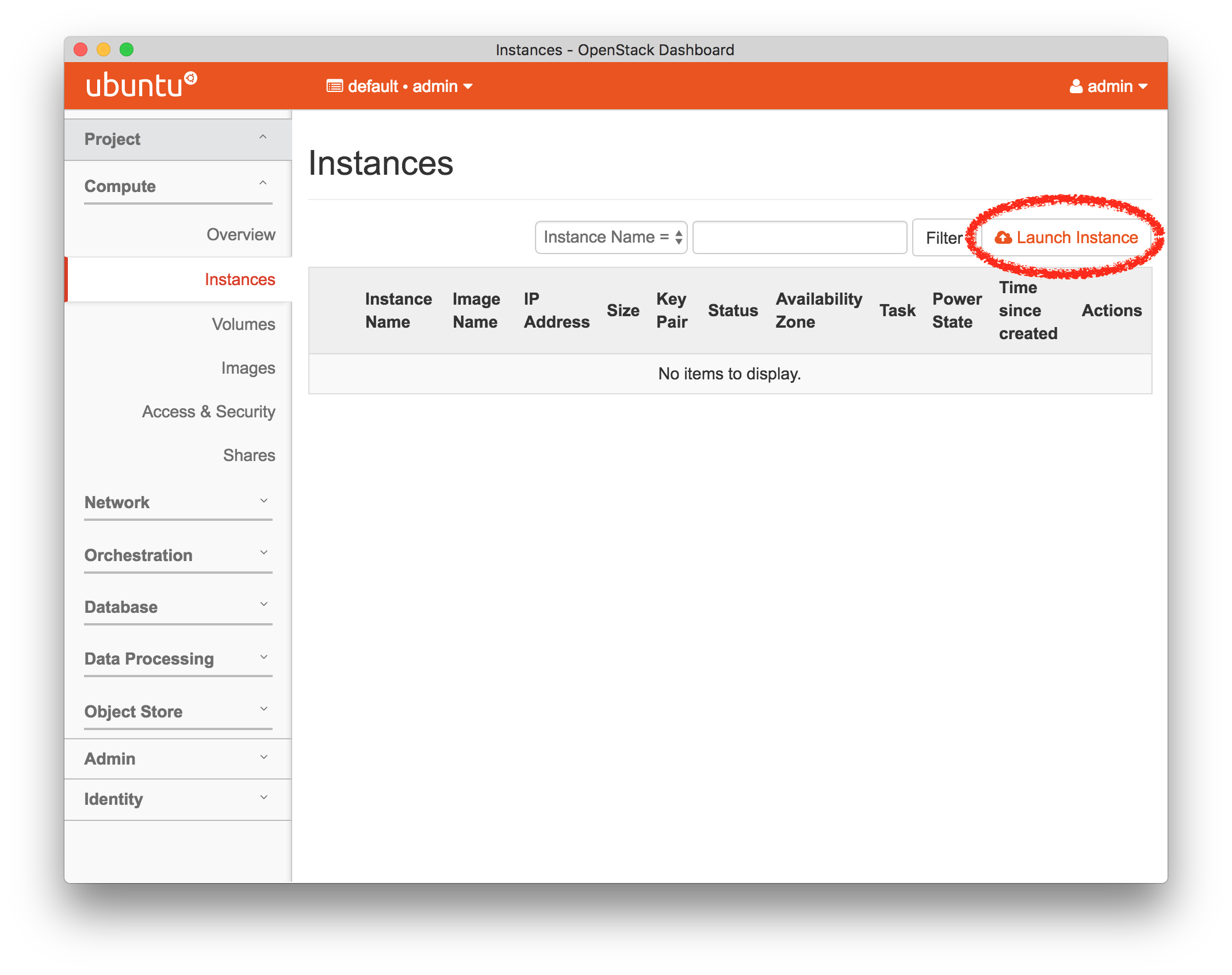
- Set Basic Settings For the InstanceThere a few settings you will need to make in order to launch your instance. These instructions are for the launch wizard in the OpenStack Mitaka, but the different release wizards are all similar in function and required information. Use the tabs in the column on the left of the launch wizard to add the required information (i.e., Details, Source, Flavor, Networks, and Key Pair), as shown in the following screenshots:
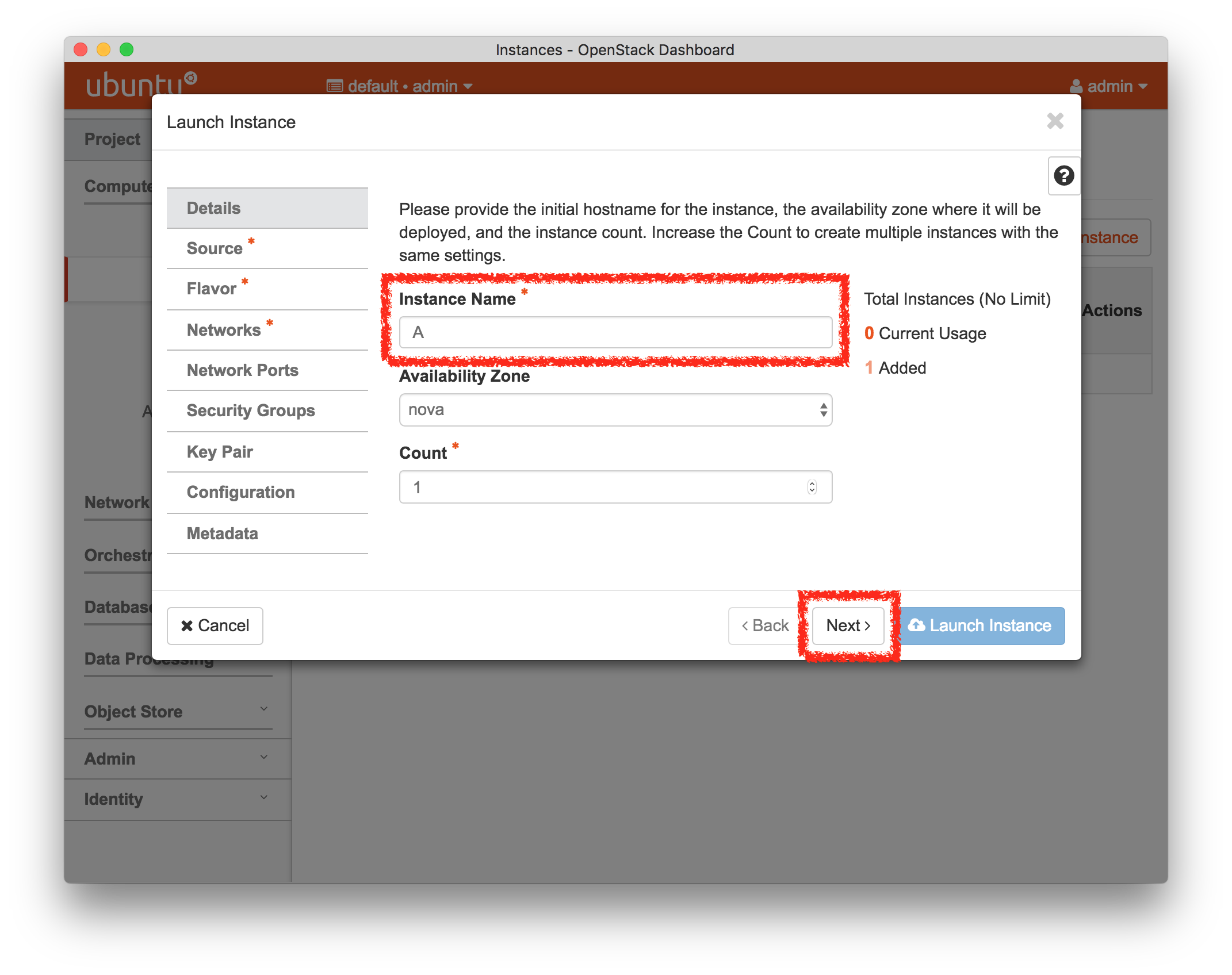
Pick any “Instance Name” you wish
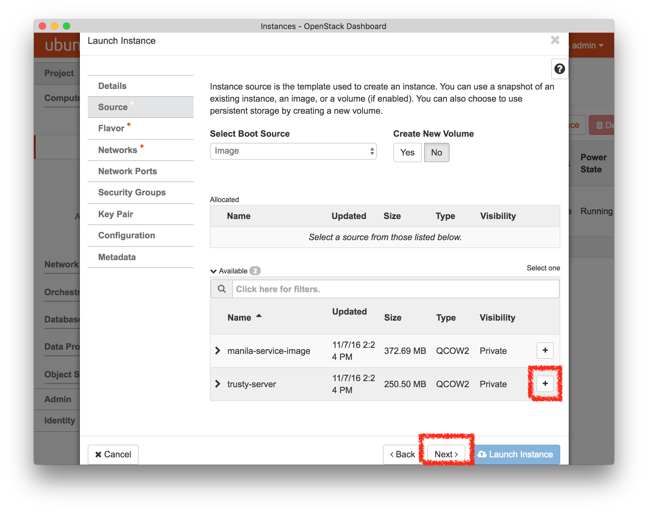
For the “Image Name”, select “trusty-server”
For the “Instance Boot Source”, select “Boot from image”
Important: If you do not see any available images, the image import script may not have finished yet; wait a few minutes, reload the page, and try again.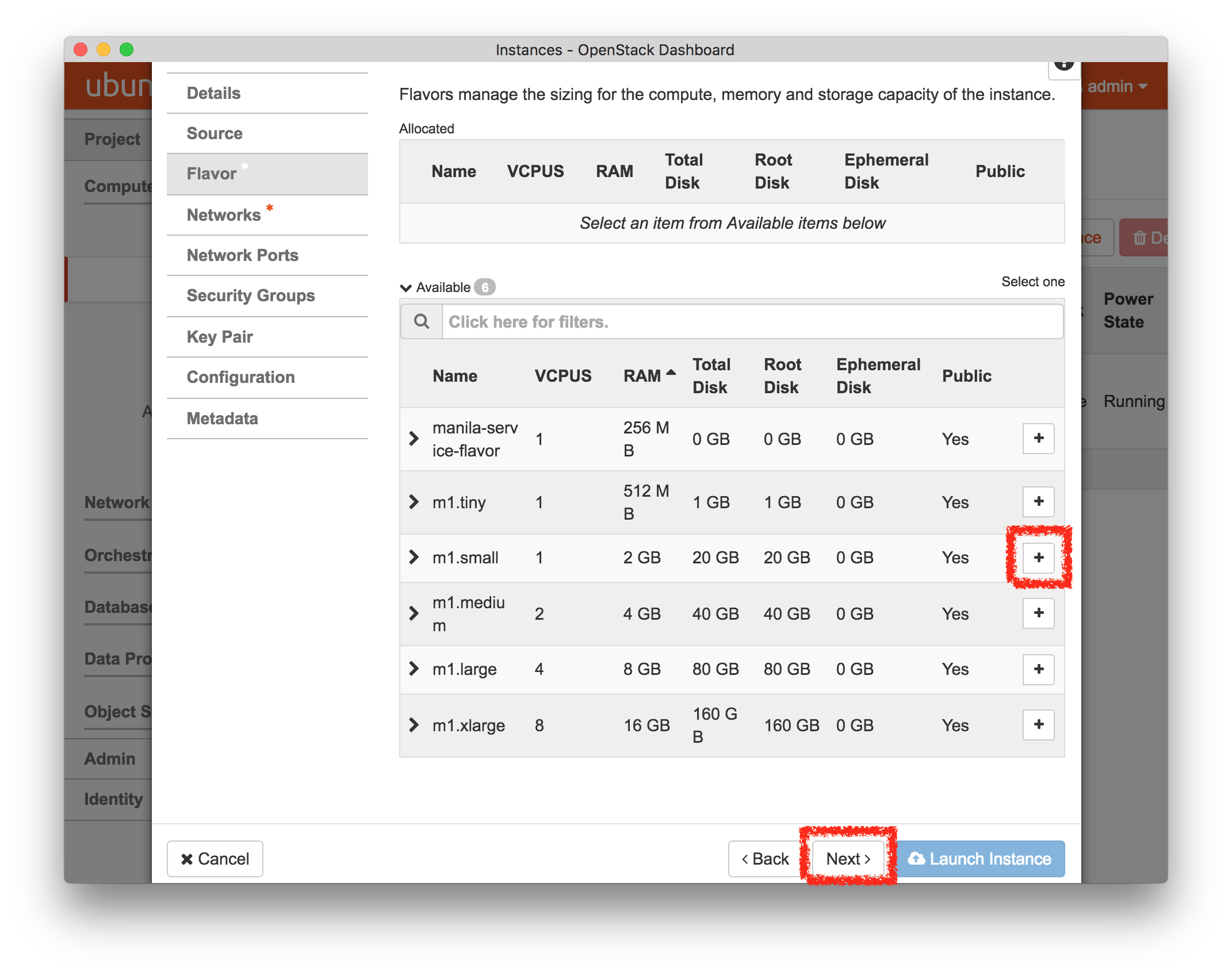
Set the “Flavor” to m1.small—
the disk for the default m1.tiny instance is too small for the image we will be using, and since we have only one compute node, we want to avoid using up too many of its resources.
- Add a Network to the InstanceIn order to be able to access your instance, you will need to give it a network. On the “Networking” tab, add the tun0-net to the list of selected networks by clicking the “+” button or dragging it up to the blue region. This will set up an internal tunneled connection within your cloud; later, we will assign a public IP address to it.
The tun0-net consists of EGRE tunnels on the CloudLab experiment network.
Important: If you are missing the Networking tab, you may have logged into the OpenStack web interface before all services were started. Unfortunately, reloading does not solve this, you will need to log out and back in.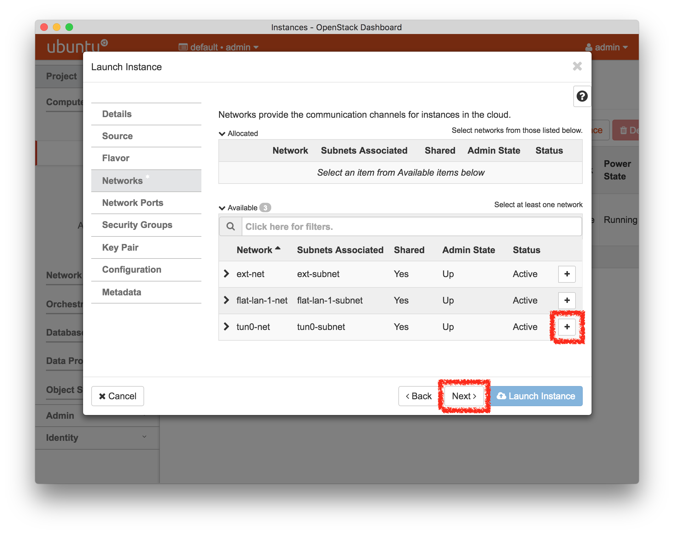
- Set an SSH KeypairOn the “Key Pair” tab (or “Access & Security” in previous versions), you will add an ssh keypair to log into your node. If you configured an ssh key in your GENI account, you should find it as one of the options in this list. You can filter the list by typing your CloudLab username, or a portion of it, into the filter box to reduce the size of the list. (By default, we load in public keys for all users in the project in which you created your experiment, for convenience – thus the list can be long.) If you don’t see your keypair, you can add a new one with the red button to the right of the list. Alternately, you can skip this step and use a password for login later.
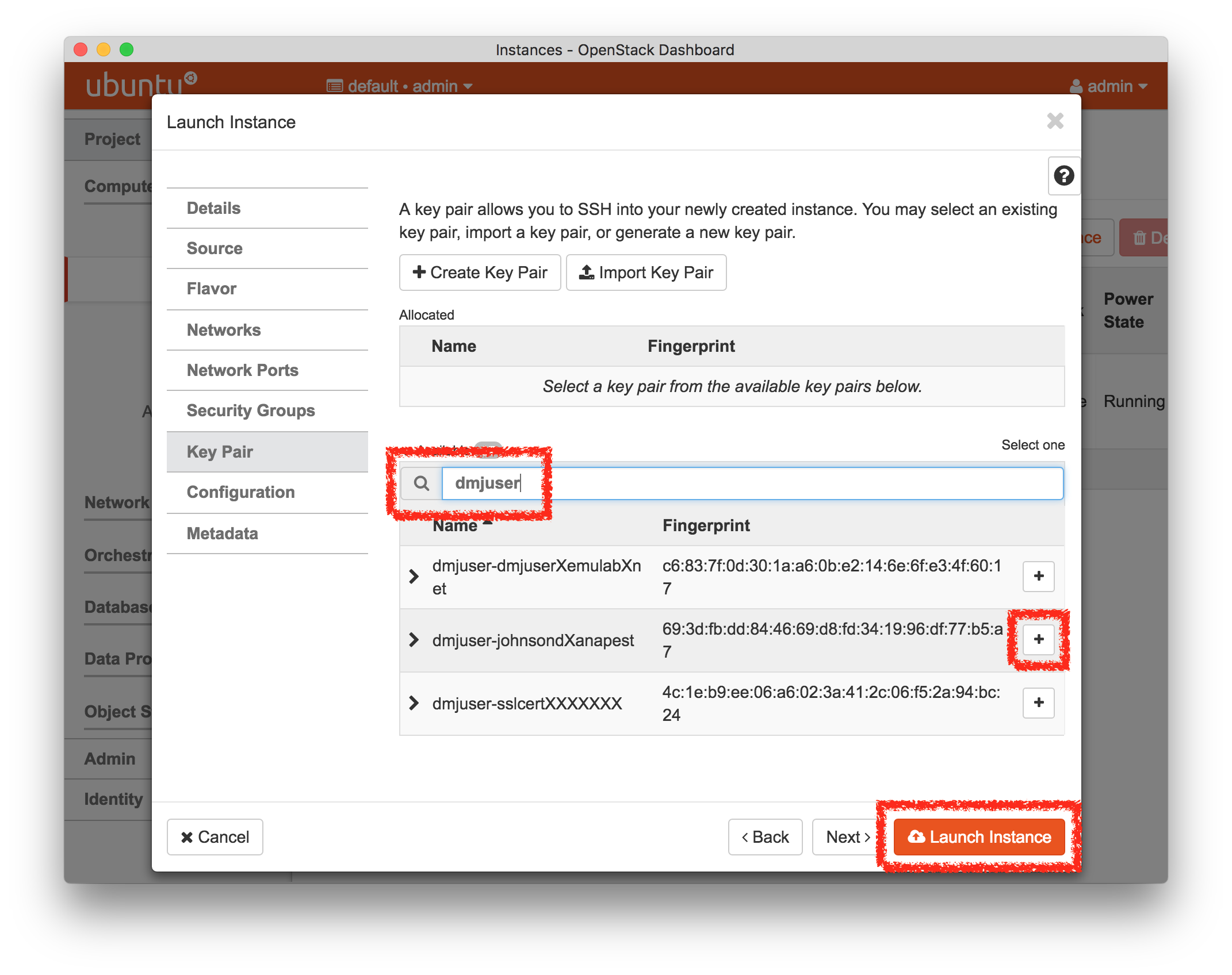
- Launch, and Wait For Your Instance to BootClick the “Launch” button on the “Key Pair” wizard page, and wait for the status on the instances page to show up as “Active”.
- Add a Public IP Address
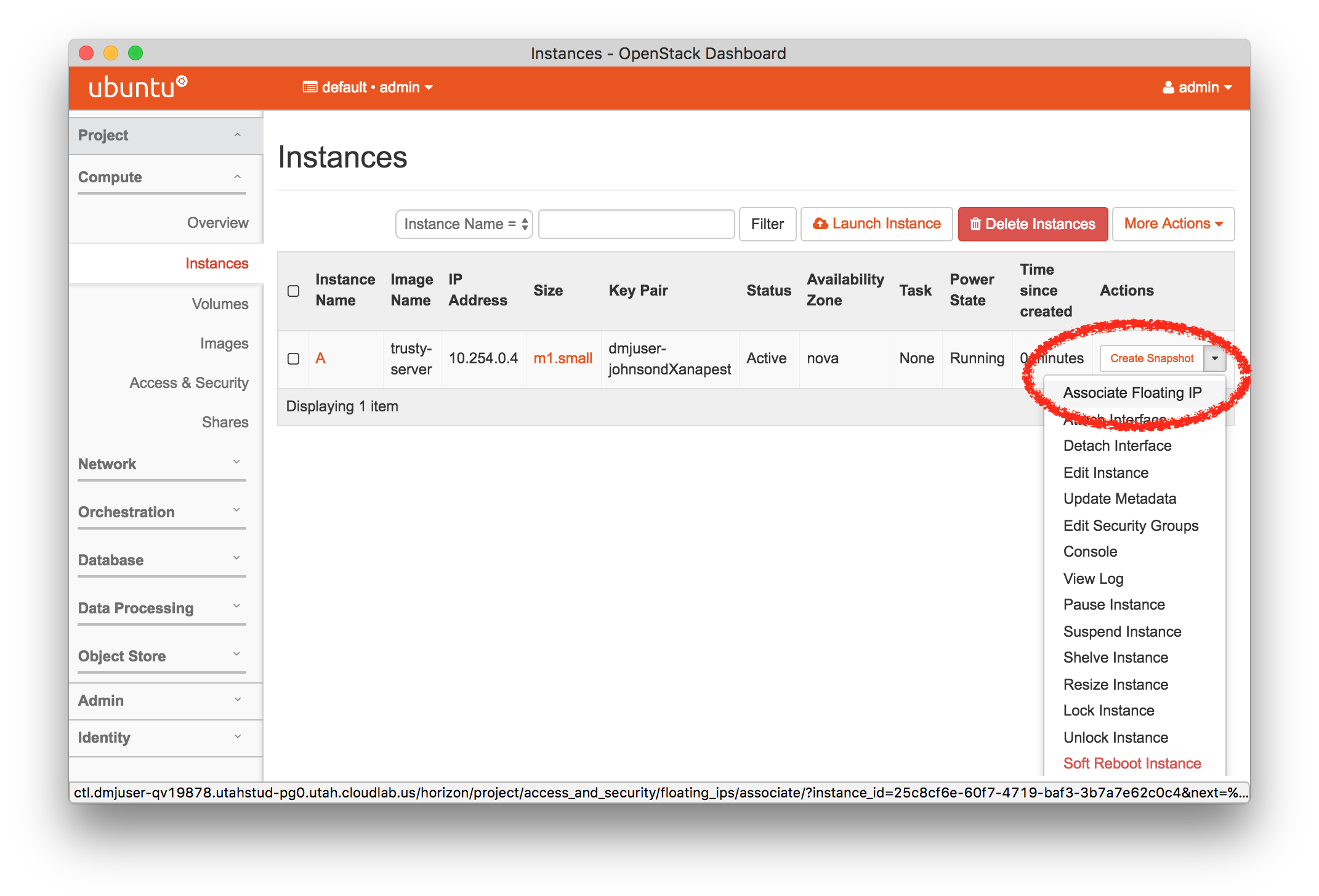 At this point, your instance is up, but it has no connection to the public Internet. From the menu on the right, select “Associate Floating IP”.
Profiles may request to have public IP addresses allocated to them; this profile requests four (two of which are used by OpenStack itself.)
On the following screen, you will need to:Press the red button to set up a new IP address
Click the “Allocate IP” button—
this allocates a new address for you from the public pool available to your cloud. Click the “Associate” button—
this associates the newly-allocated address with this instance.
The public address is tunneled by the ctl (controller) node from the control network to the experiment network. (In older OpenStack profile versions, or depending the profile parameters specified to the current profile version, the public address may instead be tunneled by the nm (network manager) node, in a split controller/network manager OpenStack deployment.)
You will now see your instance’s public address on the “Instances” page, and should be able to ping this address from your laptop or desktop.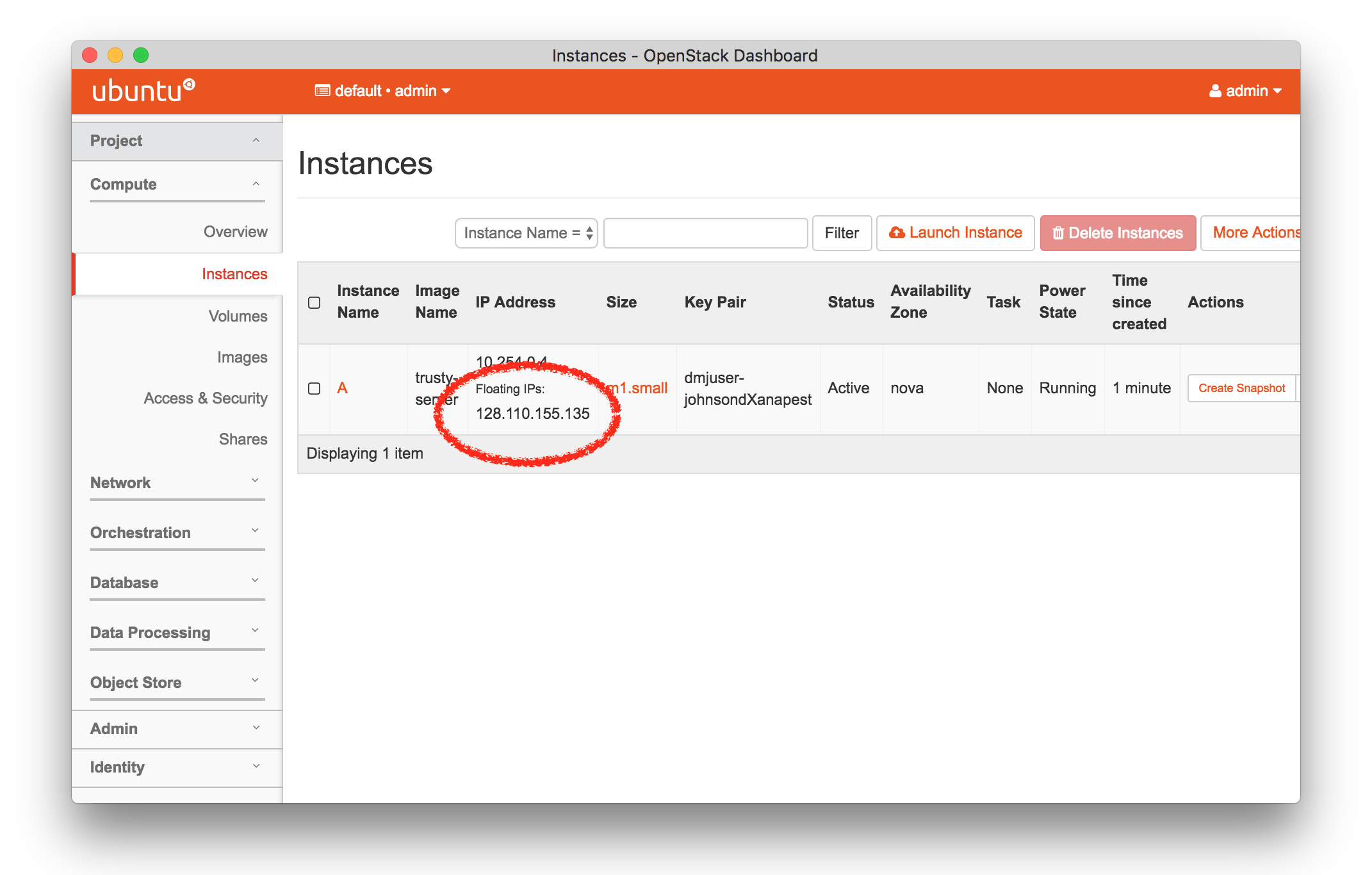
- Log in to Your InstanceYou can ssh to this IP address. Use the username ubuntu; if you provided a public key earlier, use your private ssh key to connect. If you did not set up an ssh key, use the same password you used to log in to the OpenStack web interface (shown in the profile instructions.) Run a few commands to check out the VM you have launched.
15.7 Administering OpenStack
Now that you’ve done some basic tasks in OpenStack, we’ll do a few things
that you would not be able to do as a user of someone else’s OpenStack
installation. These just scratch the surface—
15.7.1 Log Into The Control Nodes
If you want to watch what’s going on with your copy of OpenStack, you can use ssh to log into any of the hosts as described above in the List View or Web-based Shell sections. Don’t be shy about viewing or modifying things; no one else is using your cloud, and if you break this one, you can easily get another.
Some things to try:
Run ps -ef on the ctl to see the list of OpenStack services running
Run ifconfig on the ctl node (or the nm node, if your experiment has one), to see the various bridges and tunnels that have been brought to support the networking in your cloud
Run sudo virsh list --all on cp1 to see the VMs that are running
15.7.2 Reboot the Compute Node
Since you have this cloud to yourself, you can do things like reboot or re-image nodes whenever you wish. We’ll reboot the cp1 (compute) node and watch it through the serial console.
- Open the serial console for cp1On your experiment’s CloudLab status page, use the action menu as described in Actions to launch the console. Remember that you may have to click to focus the console window and hit enter a few times to see activity on the console.
- Reboot the nodeOn your experiment’s CloudLab status page, use the action menu as described in Actions to reboot cp1. Note that in the topology display, the box around cp1 will turn yellow while it is rebooting, then green again when it has booted.
- Watch the node boot on the consoleSwitch back to the console tab you opened earlier, and you should see the node starting its reboot process.
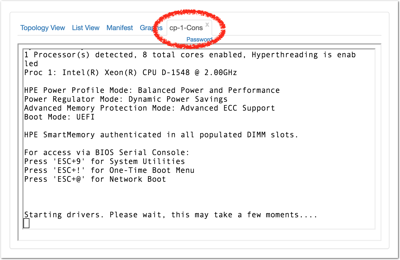
- Check the node status in OpenStackYou can also watch the node’s status from the OpenStack Horizon web interface. In Horizon, select “Hypervisors” under the “System” menu, and switch to the “Compute Host” tab.
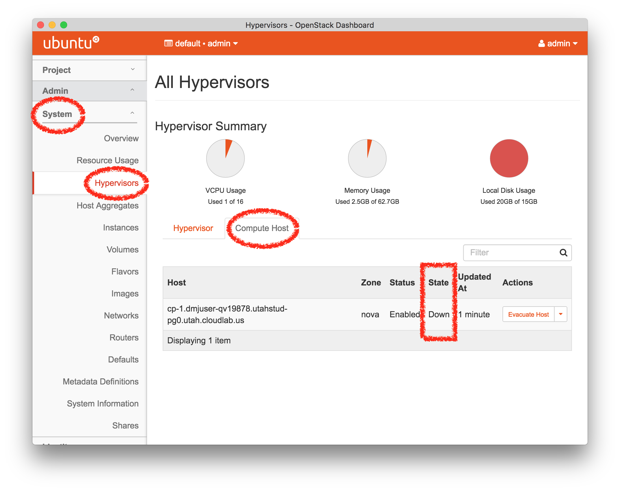 Note: This display can take a few minutes to notice that the node has gone down, and to notice when it comes back up. Your instances will not come back up automatically; you can bring them up with a “Hard Reboot” from the “Admin -> System ->Instances” page.
15.8 Terminating the Experiment
Resources that you hold in CloudLab are real, physical machines and are therefore limited and in high demand. When you are done, you should release them for use by other experimenters. Do this via the “Terminate” button on the CloudLab experiment status page.
Note: When you terminate an experiment, all data on the nodes is lost, so make sure to copy off any data you may need before terminating.
If you were doing a real experiment, you might need to hold onto the nodes for longer than the default expiration time. You would request more time by using the “Extend” button the on the status page. You would need to provide a written justification for holding onto your resources for a longer period of time.
15.9 Taking Next Steps
Now that you’ve got a feel for for what CloudLab can do, there are several things you might try next:
Create a new project to continue working on CloudLab past this tutorial
Try out some profiles other than OpenStack (use the “Change Profile” button on the “Start Experiment” page)
Read more about the basic concepts in CloudLab
Try out different hardware
Learn how to make your own profiles
16 CloudLab Chef Tutorial
This tutorial will walk you through the process of creating and using an instance of the Chef configuration management system on CloudLab.
Chef is both the name of a company and the name of a popular modern configuration management system written in Ruby and Erlang. A large variety of tutorials, articles, technical docs and training opportunities is available at the Chef official website. Also, refer to the Customer Stories page to see how Chef is used in production environments, including very large installations (e.g., at Facebook, Bloomberg, and Yahoo!).
16.1 Objectives
In the process of taking this tutorial, you will learn to:
Create your own instance of Chef using a pre-defined profile
Explore profile parameters allowing to customize components of your Chef deployments
Access monitoring and management capabilities provided by Chef
- Use Chef to perform two exercises:
Install and configure NFS, the Network File System, on experiment nodes
Install and configure an instance of the Apache web server, as well as run a benchmark against it
Terminate your experiment
Learn where to get more information
16.2 Motivation
This tutorial will demonstrate how experiments can be managed on CloudLab, as well as show how experiment resources can be administered using Chef. By following the instructions provided below, you will learn how to take advantage of the powerful features of Chef for configuring multi-node software environments. The exercises included in this tutorial are built around simple but realistic configurations. In the process of recreating these configurations on nodes running default images, you will explore individual components of Chef and follow the configuration management workflow applicable to more complex configurations and experiments.
16.3 Prerequisites
This tutorial assumes that:
- You have an existing account on either:
CloudLab (Instructions for getting an account can be found here.)
The GENI portal. (Instructions for getting an account can be found here.)
16.4 Logging In
If you have signed up for an account at the CloudLab website, simply open https://www.cloudlab.us/ in your browser, click the “Log In” button, enter your username and password.
16.5 Launching Chef Experiments
Once you have logged in to CloudLab, you will “instantiate” a “profile” to create an experiment. (An experiment in CloudLab is similar to a “slice” in GENI.) Profiles are CloudLab’s way of packaging up configurations and experiments so that they can be shared with others. Each experiment is separate: the experiment that you create for this tutorial will be an instance of a profile provided by the facility, but running on resources that are dedicated to you, which you have complete control over. This profile uses local disk space on the nodes, so anything you store there will be lost when the experiment terminates.
The Chef cluster we are building in this tutorial is very small, but CloudLab has large clusters that can be used for larger-scale experiments.
For this tutorial, we will use a profile that launches a Chef cluster —
See this manual’s section on profiles for more information about how they work.
- Start ExperimentAfter logging in, you are taken to your main status dashboard. Select “Start Experiment” from the “Experiments” menu.
- Select a profileBy default, the “Start an Experiment” page suggests launching the OpenStack profile which is discribed in detail in the OpenStack tutorial.Go to the list of available profile by clicking “Change Profile”:
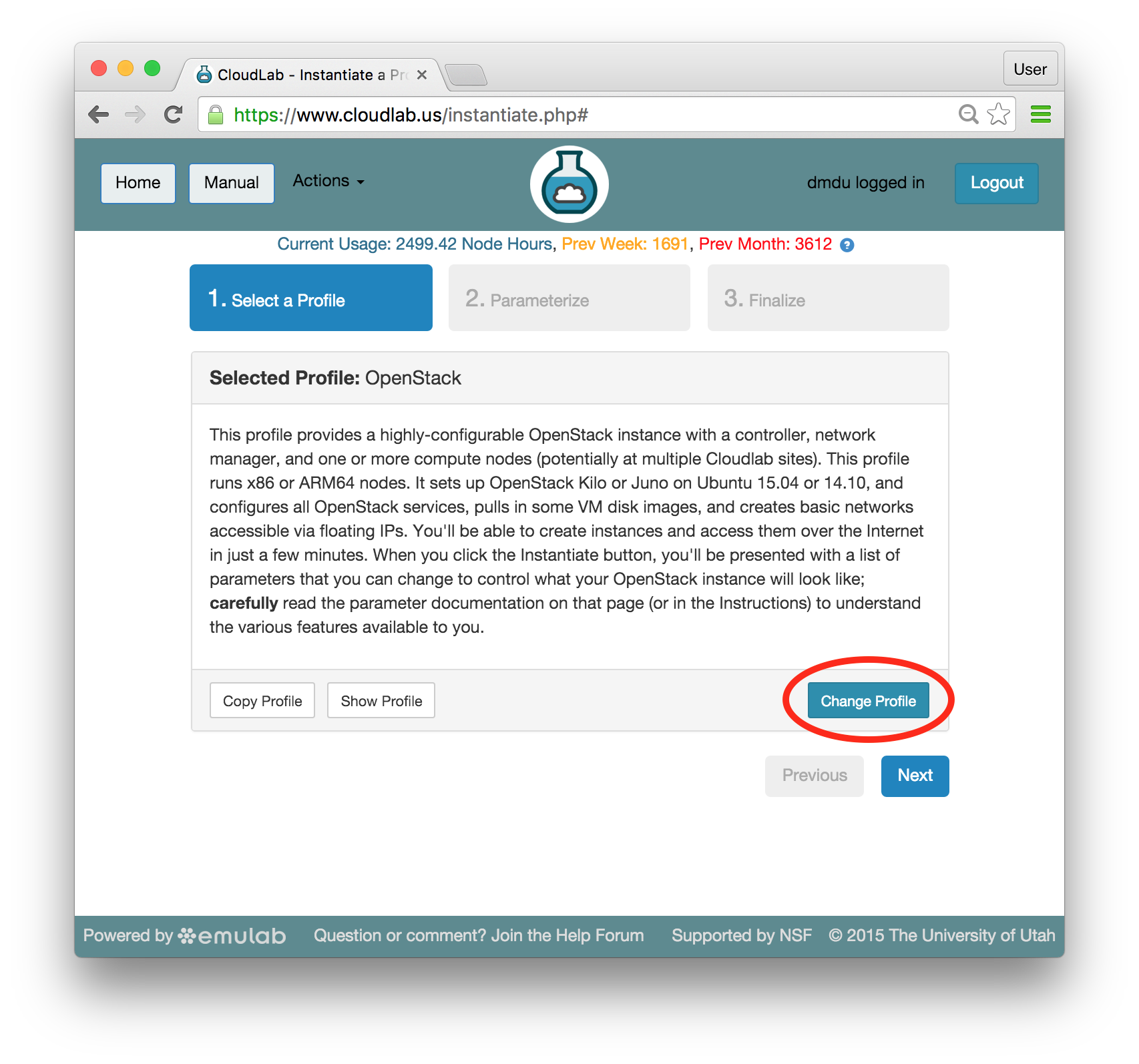 Find the profile by typing ChefCluster in the search bar. Then, select the profile with the specified name in the list displayed below the search bar. A 2-node preview should now be shown along with high-level profile information. Click “Select Profile” at the bottom of the page:
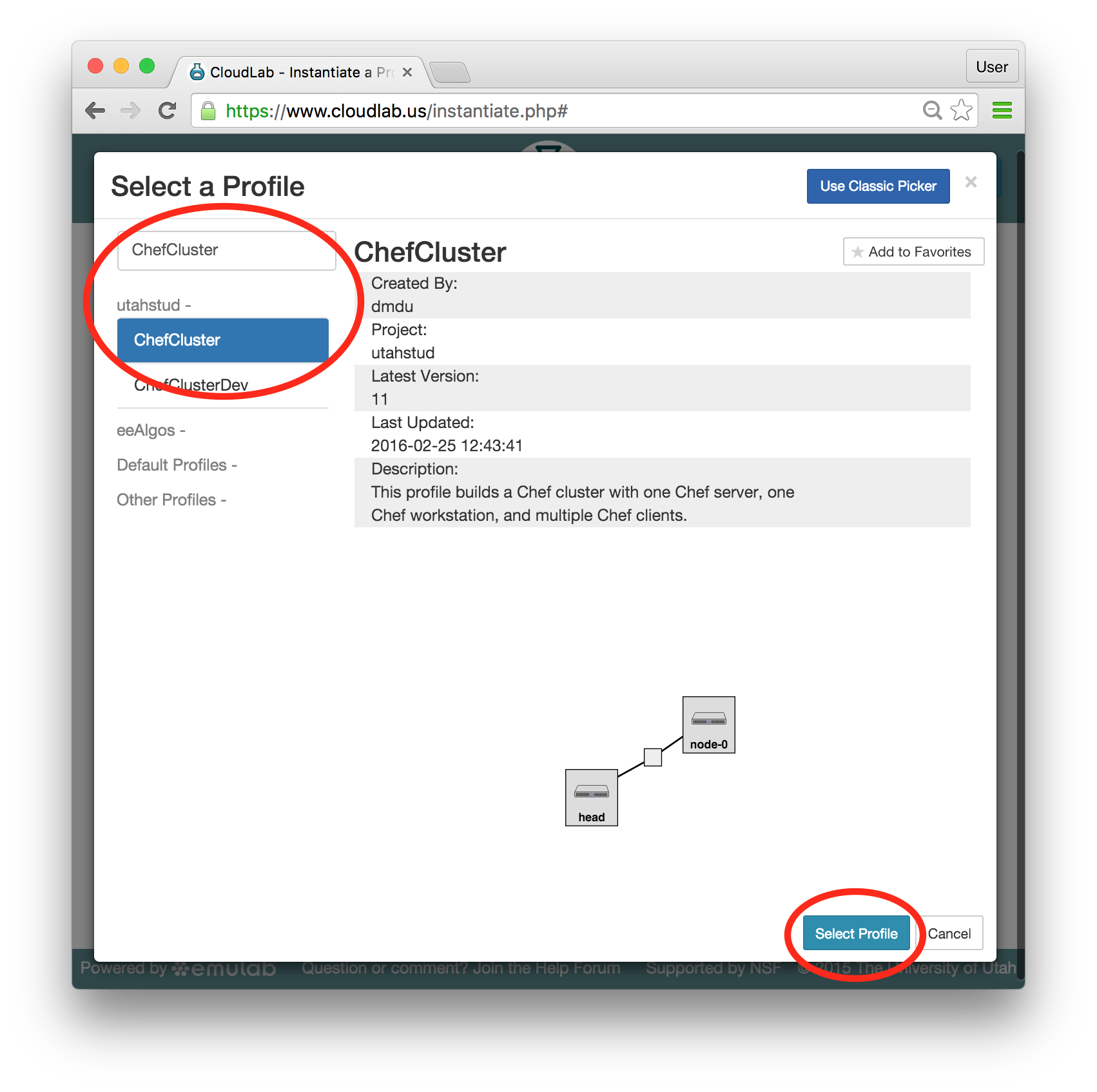 After you select the correct profile, click “Next”:
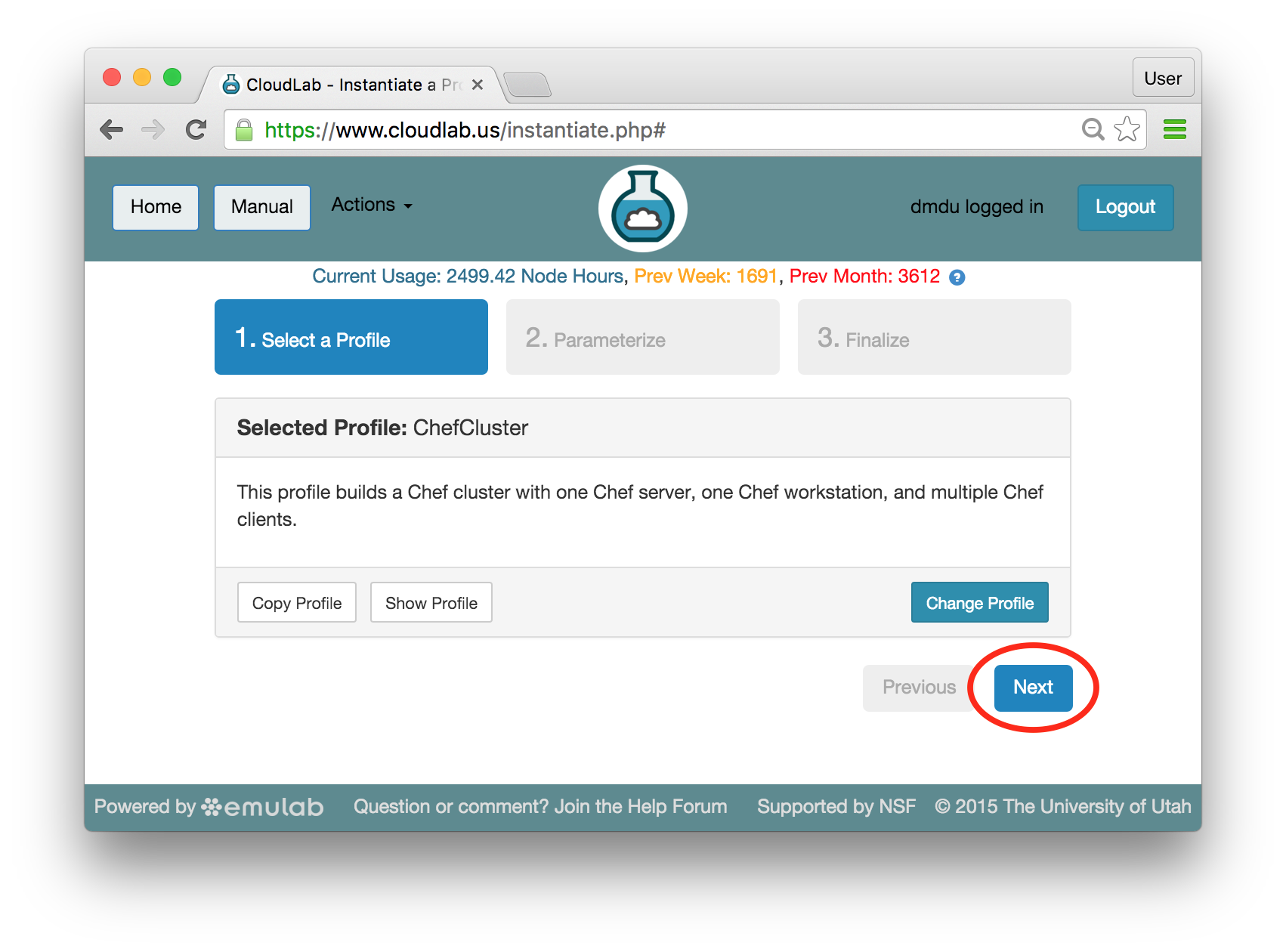
- Set parametersProfiles in CloudLab can have parameters that affect how they are configured; for example, this profile has parameters that allow you to set the number of client nodes, specify the repository with the infrastructure code we plan to use, obtain copies of the application-specific infrastructure code developed by the global community of Chef developers, etc.For this tutorial, we will leave all parameters at their defaults and just click “Next”.
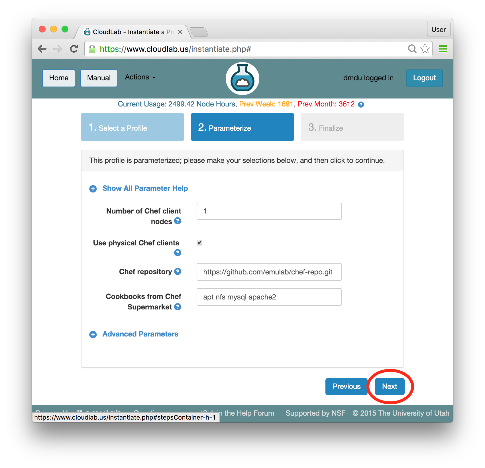
- Choose experiment nameYou may optionally give your experiment a meaningful name, e.g., “chefdemo”. This is useful if you have many experiments running at once.
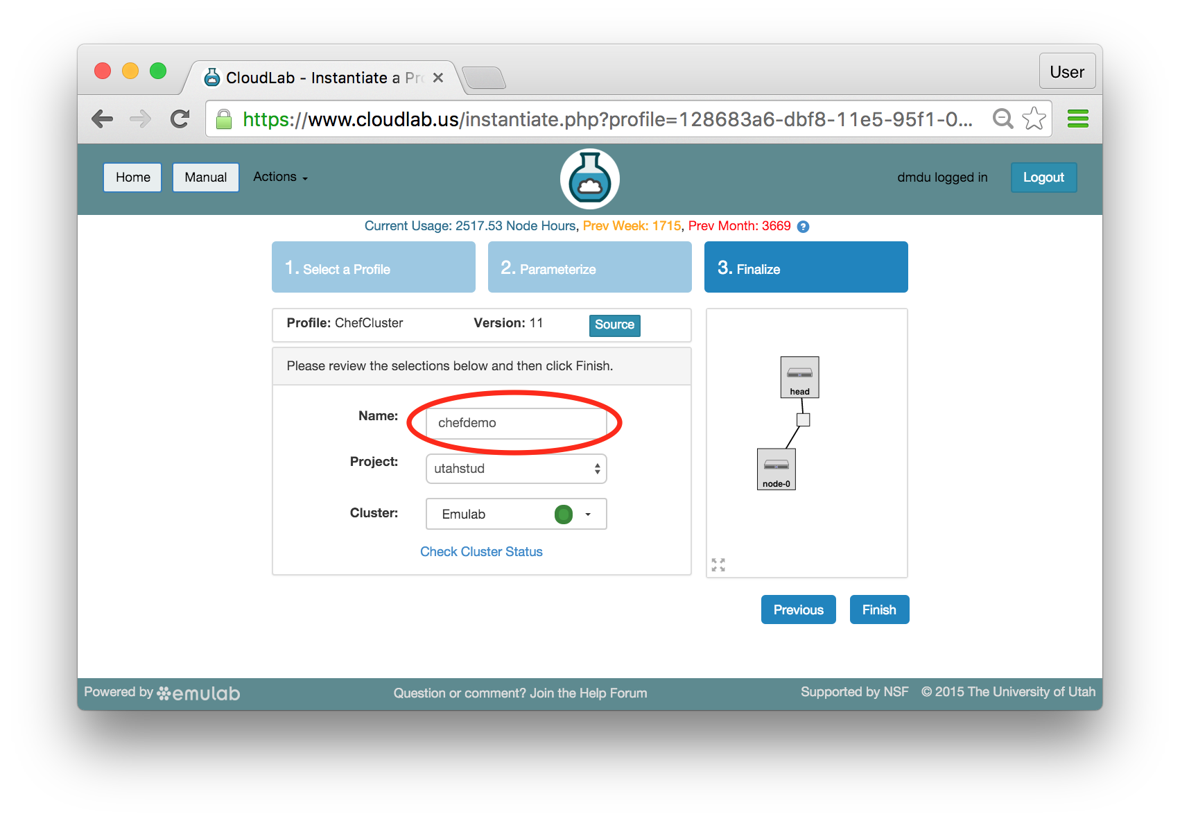
- Select a clusterCloudLab has multiple clusters available to it. Some profiles can run on any cluster, some can only run on specific ones due to specific hardware constraints. ChefCluster can only run on the x86-based clusters. This excludes the CloudLab Utah cluster which is built on ARMv8 nodes. Refer to the Hardware section for more information.Note: If you are at an in-person tutorial, the instructor will tell you which cluster to select. Otherwise, you may select any compatible and available cluster.
The dropdown menu for the clusters shows you both the health (outer ring) and available resources (inner dot) of each cluster. The “Check Cluster Status” link opens a page (in a new tab) showing the current utilization of all CloudLab clusters.
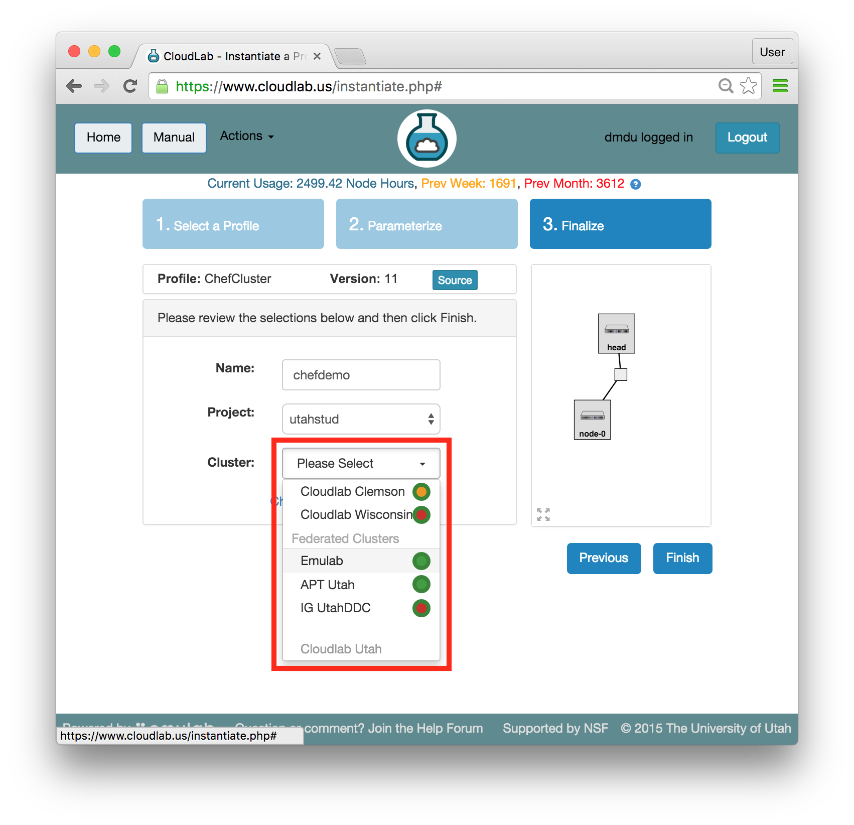
- Click Finish!When you click the “Finish” button, CloudLab will start provisioning the resources that you requested on the cluster that you selected.
- @(tb) instantiates your profileCloudLab will take a few minutes to bring up your experiment, as many things happen at this stage, including selecting suitable hardware, loading disk images on local storage, booting bare-metal machines, re-configuring the network topology, etc. While this is happening, you will see the topology with yellow node icons:
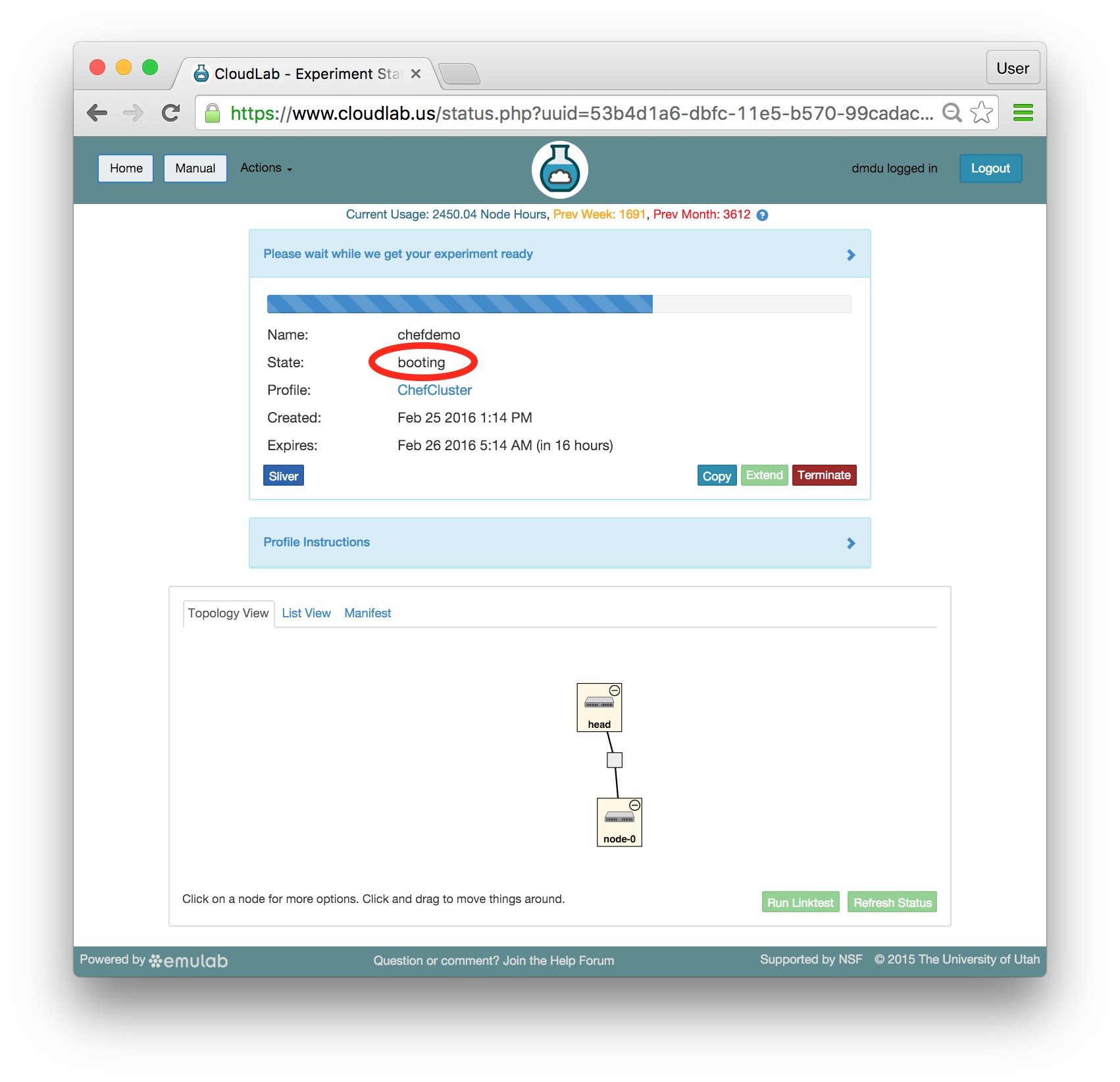
Provisioning is done using the GENI APIs; it is possible for advanced users to bypass the CloudLab portal and call these provisioning APIs from their own code. A good way to do this is to use the geni-lib library for Python.
As soon as a set of resources have been assigned to you, you will see details about them if you switch to the "List View" tab (though you will not be able to log in until they have gone through the process of imaging and booting.) While you are waiting for your resources to become available, you may want to have a look at the CloudLab user manual, or use the “Sliver” button to watch the logs of the resources (“slivers”) being provisioned and booting. - Your resources are ready!Shortly, the web interface will report the state as “Booted”.
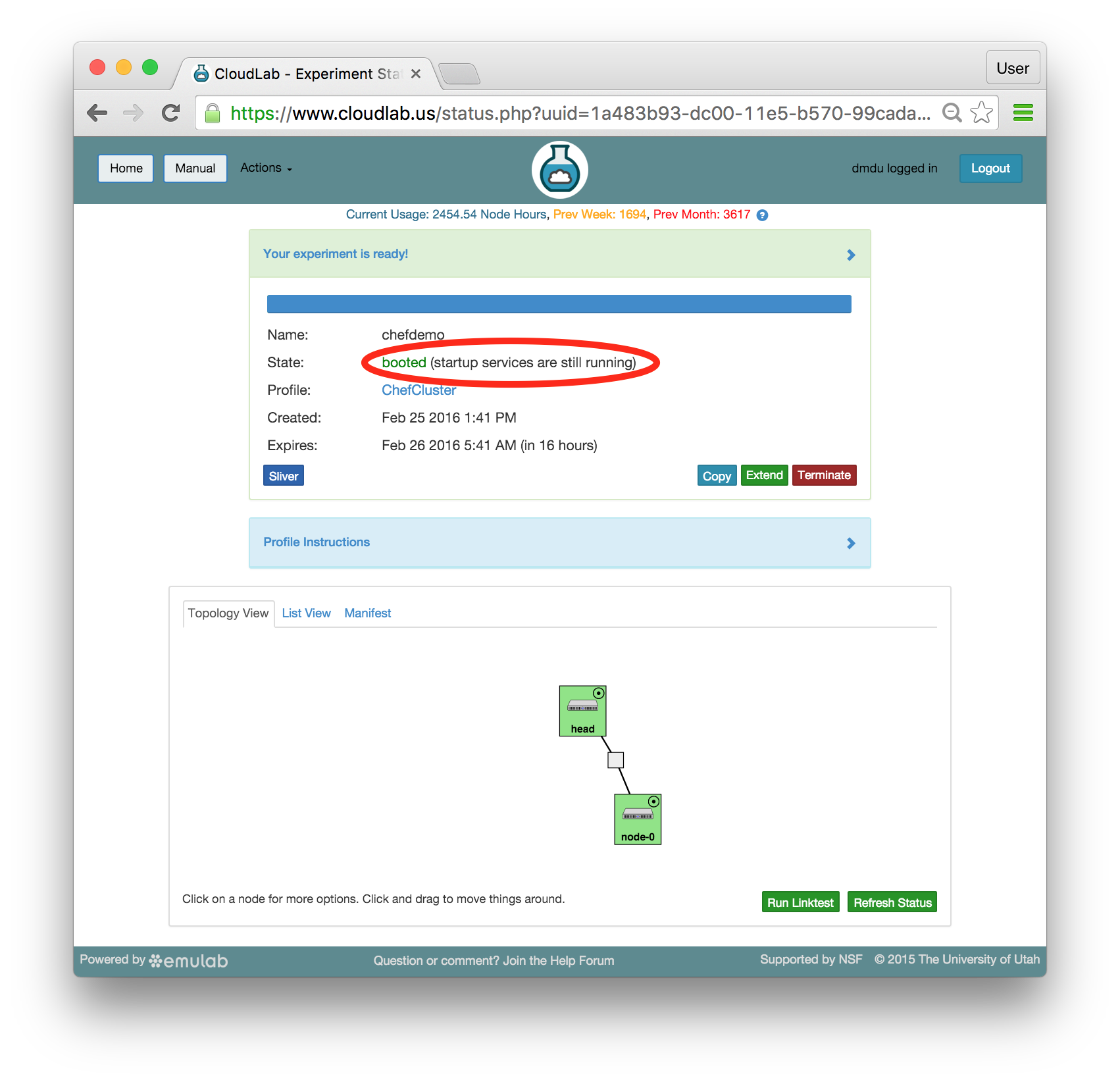 Important: A “Booted” status indicates that resources are provisioned and booted; this particular profile runs scripts to complete the Chef setup, and it will be a few more minutes before Chef becomes fully functional. You will be able to tell that the configuration process has finished when the status changes from “Booted” to “Ready”. Until then, you will likely see that the startup scripts (i.e. programs that run at the beginning of the experiment to set it up) run longer on head than on node-0 —
a lot more work is required to install the Chef server than the client. In the Topology View tab, mouse over the circle in the head’s icon, to confirm the current state of the node. 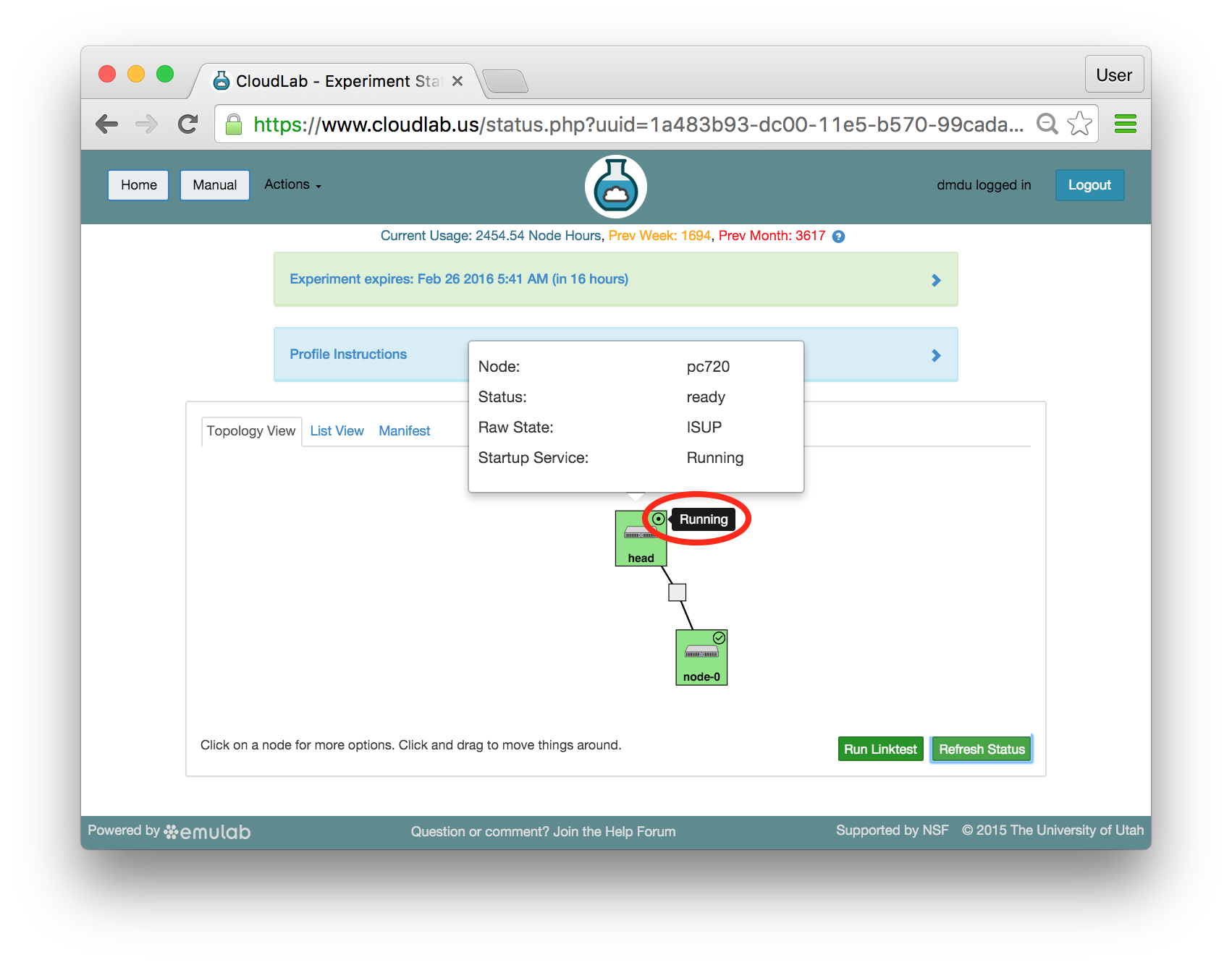
16.6 Exploring Your Experiment
While the startup scripts are still running, you will have a few minutes to look at various parts of the CloudLab experiment page and learn what resources you now have access to and what you can do with them.
16.6.1 Experiment Status
The panel at the top of the page shows the status of your experiment —
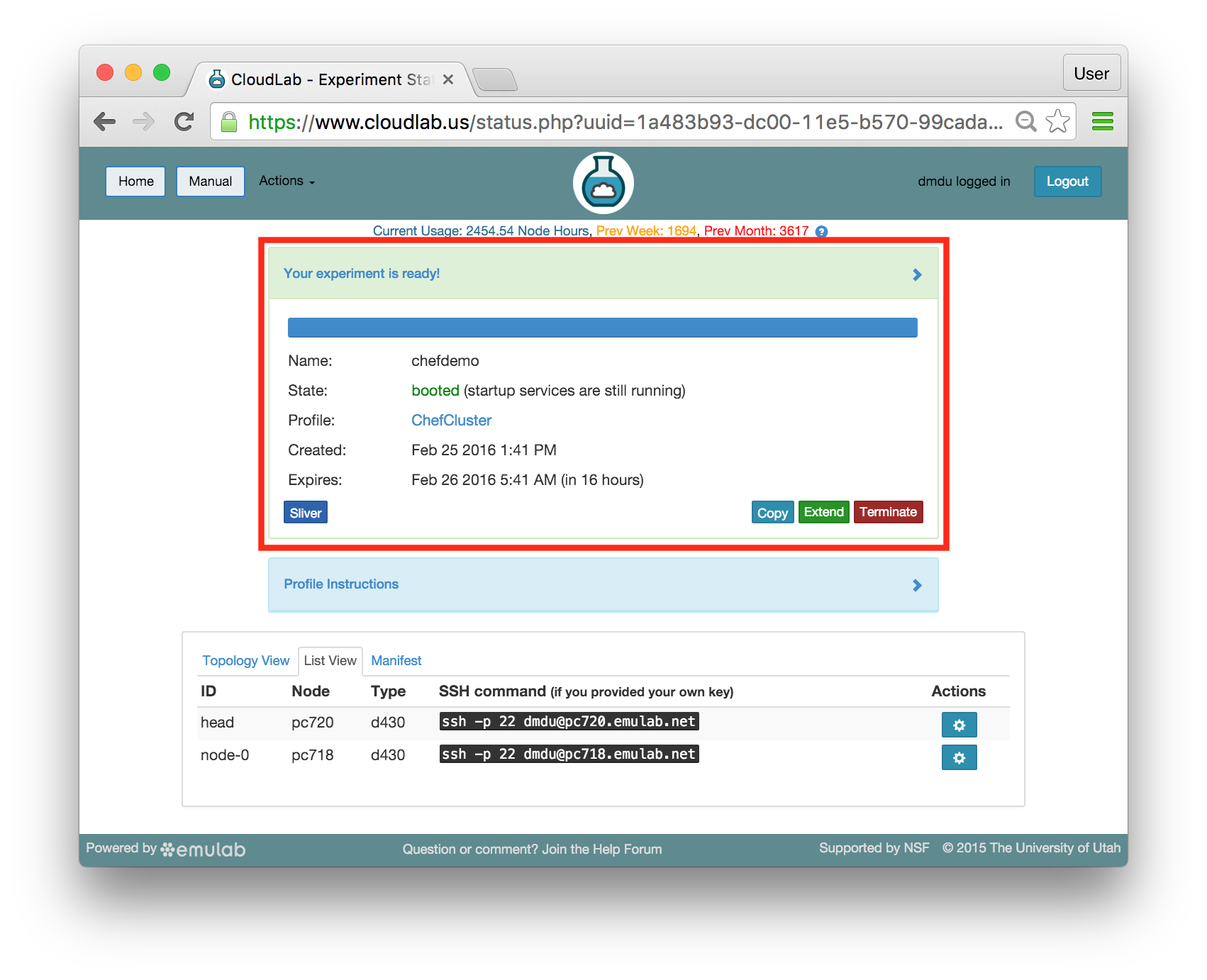
Note that the default lifetime for experiments on CloudLab is less than a day; after this time, the resources will be reclaimed and their disk contents will be lost. If you need to use them for longer, you can use the “Extend” button and provide a description of why they are needed. Longer extensions require higher levels of approval from CloudLab staff. You might also consider creating a profile of your own if you might need to run a customized environment multiple times or want to share it with others.
You can click on the title of the panel to expand or collapse it.
16.6.2 Profile Instructions
Profiles may contain written instructions for their use. Clicking on the title
of the “Profile Instructions” panel will expand or collapse it. In this
case, the instructions provide a link to the Chef server web console.
(Don’t click on the link yet —
Also, notice the list of private and public hostnames of the experiment nodes included in the instructions. You will use the public hostnames (shown in bold) in the exercise with the Apache web server and apache benchmark.

16.6.3 Topology View
We have already used the topology viewer to see the node status; let’s take a closer look at the topology of this experiment. This profile has two nodes connected by a 10 Gigabit LAN, which is represented by a gray box in the middle of the topology. The names given for each node are the names assigned as part of the profile; this way, every time you instantiate a profile, you can refer to the nodes using the same names, regardless of which physical hardware was assigned to them. The green boxes around each node indicate that they are up; click the “Refresh Status” button to initiate a fresh check.
You can also run several networking tests by clicking the “Run Linktest” button at the bottom of the page. The available tests include:
Level 1 —
Connectivity and Latency Level 2 —
Plus Static Routing Level 3 —
Plus Loss Level 4 —
Plus Bandwidth Higher levels will take longer to complete and require patience.

If an experiment has startup services, their statuses are indicated by small icons in the upper right corners of the node icons. You can mouse over this icon to see a description of the current status. In this profile, the startup services on the client node(s), such as node-0, typically complete quickly, but the scripts on head take much longer. The screenshot above shows the state of the experiment when all startup scripts complete.
It is important to note that every node in CloudLab has at least two network interfaces: one “control network” that carries public IP connectivity, and one “experiment network” that is isolated from the Internet and all other experiments. It is the experiment net that is shown in this topology view. You will use the control network to ssh into your nodes, interact with their web interfaces, etc. This separation gives you more freedom and control in the private experiment network, and sets up a clean environment for repeatable research.
16.6.4 List View
The list view tab shows similar information to the topology view, but in a different format. It shows the identities of the nodes you have been assigned, and the full ssh command lines to connect to them. In some browsers (those that support the ssh:// URL scheme), you can click on the SSH commands to automatically open a new session. On others, you may need to cut and paste this command into a terminal window. Note that only public-key authentication is supported, and you must have set up an ssh keypair on your account before starting the experiment in order for authentication to work.
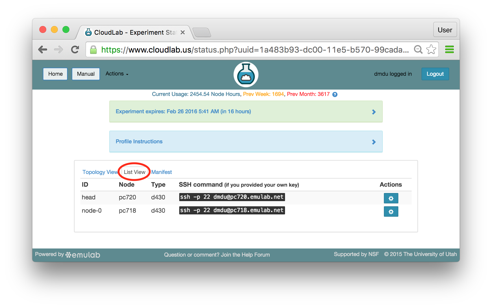
16.6.5 Manifest View
The final default tab shows a manifest detailing the hardware that has been assigned to you. This is the “request” RSpec that is used to define the profile, annotated with details of the hardware that was chosen to instantiate your request. This information is available on the nodes themselves using the geni-get command, enabling you to do rich scripting that is fully aware of both the requested topology and assigned resources.
Most of the information displayed on the CloudLab status page comes directly from this manifest; it is parsed and laid out in-browser.
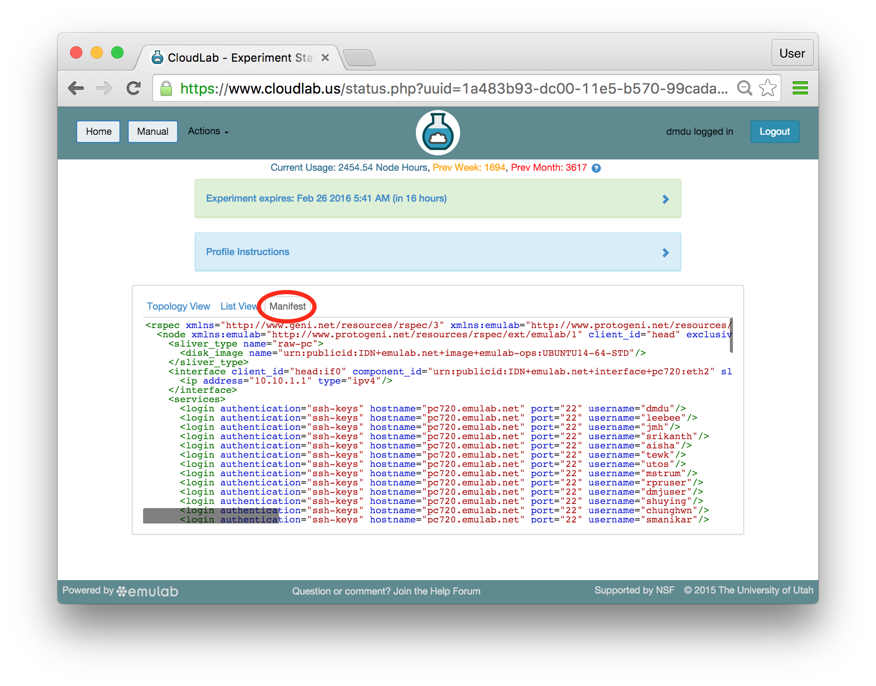
16.6.6 Actions
In both the topology and list views, you have access to several actions that you may take on individual nodes. In the topology view, click on the node to access this menu; in the list view, it is accessed through the icon in the “Actions” column. Available actions include rebooting (power cycling) a node, and re-loading it with a fresh copy of its disk image (destroying all data on the node). While nodes are in the process of rebooting or re-imaging, they will turn yellow in the topology view. When they have completed, they will become green again. The shell action is described in more detail below and will be used as the main method for issuing commands on the experiment nodes throughout this tutorial.
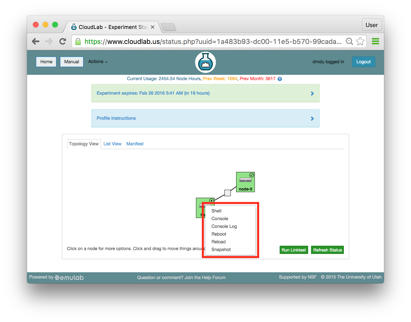
16.7 Brief Introduction to Chef
While the startup scripts are running, let’s take a quick look at the architecture of a typical Chef intallation. The diagram provided at the official Overview of Chef page demonstrates the relationships between individual Chef components. While there is a number of optional, advanced components that we don’t use in this tutorial, it is worth noting the following:
Chef clients can run on a variety of resources: virtual and physical servers, cloud instances, storage and networking devices, containers, etc. All clients connect and listen to the central, infrastructure-wide Chef server.
The Chef server has a web interface. The server manages cookbooks, which are fundamental units of configuration management that define configurations and contain everything that is required to instantiate those configurations. Additionally, the server manages run lists, which can be viewed as mappings between collections of cookbooks and the clients on which they need to execute.
A workstation represents a machine from which a Chef administrator connects to and controls the server. It typically has a copy of chef-repo, the repository which contains cookbooks and other code artifacts. The administrator modifies cookbooks locally and submits them to the server to make them available to all clients.
Recipes, shown next to cookbooks on the workstation, are the "building blocks" from which cookbooks are assembled. Recipes can be viewed as individual scripts accomplishing specific fine-grained tasks, such as create a user, install a package, clone a repository, configure a network interface, etc. Cookbooks, which include one or more recipes, are responsible for "bigger" tasks: install and configure a database, install and run a web server, and so on.
Another type of Chef code artifacts (not shown in the diagram) is called role. A role can include one or more cookbooks and specific recipes (each cookbook and recipe can be used in several roles if necessary). Roles typically define complete node configurations; for instance, in a simple case, one role corresponds to a master node on a cluster with a set of specific services, while another role defines how the rest of the cluster nodes, so-called “worker” nodes, should be configured. After being created on the workstation, these roles are submitted to the server by the administrator and then assigned to specific nodes via the run lists.
In the experiment we have launched, head runs all three: the server, the workstation, and the client
(there is no conflict between these components), while node-0 runs only the client. If this profile is instantiated
with the arbitrary number N of clients, there will be N “client-only” nodes
named node-0,node-1,...,node-(N-1).
Another profile parameter allows choosing the repository from which chef-repo is cloned;
by default, it points to emulab/chef-repo.
The startup scrips in this profile also obtain and install copies of public cookbooks
hosted at the respository called Supermarket.
Specifically, the exercises in this tutorial rely on the nfs
and apache2 cookbooks —
16.8 Logging in to the Chef Web Console
As soon as the startup scripts complete, you will likely recieve an email confirming that Chef is installed and operational.
Dear User, |
|
Chef server and workstataion should now be |
installed on head.chefdemo.utahstud.emulab.net. |
|
To explore the web management console, copy |
this hostname and paste it into your browser. |
Installation log can be found at /var/log/init-chef.log |
on the server node. |
|
To authenticate, use the unique credentials |
saved in /root/.chefauth on the server node. |
|
Below are several Chef commands which detail the launched experiment: |
|
# chef -v |
Chef Development Kit Version: 0.7.0 |
chef-client version: 12.4.1 |
berks version: 3.2.4 |
kitchen version: 1.4.2 |
|
# knife cookbook list |
apache2 3.1.0 |
apt 2.9.2 |
emulab-apachebench 1.0.0 |
emulab-nfs 0.1.0 |
... |
nfs 2.2.6 |
|
# knife node list |
head |
node-0 |
|
# knife role list |
apache2 |
apachebench |
... |
nfs |
|
# knife status -r |
1 minute ago, head, [], ubuntu 14.04. |
0 minutes ago, node-0, [], ubuntu 14.04. |
|
Happy automation with Chef! |
In some cases, you will not be able to see this email —
When you receive this email or see in the topology viewer that the startup scripts completed, you can proceed to the following step.
16.8.1 Web-based Shell
CloudLab provides a browser-based shell for logging into your nodes, which is accessed through the action menu described above. While this shell is functional, it is most suited to light, quick tasks; if you are going to do serious work, on your nodes, we recommend using a standard terminal and ssh program.
This shell can be used even if you did not establish an ssh keypair with your account.
Three things of note:
Your browser may require you to click in the shell window before it gets focus.
Depending on your operating system and browser, cutting and pasting into the window may not work. If keyboard-based pasting does not work, try right-clicking to paste.
The recommended browsers are Chrome and Firefox. The web-based shell does not work reliably in Safari. It is not guaranteed that it works smoothly in other browsers.
Create a shell tab for head by choosing “Shell” in the Actions menu for head in either the topology or the list view. The new tab will be labeled “head”. It will allow typing shell commands and executing them on the node. All shell commands used throughout this tutorial should be issued using this shell tab.
While you are here, switch to the root user by typing:
sudo su - |
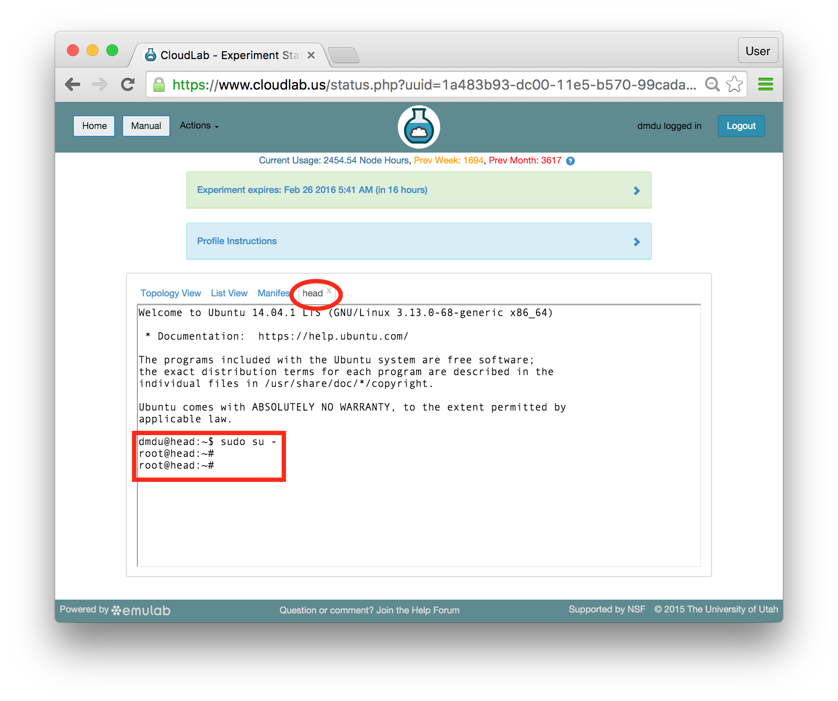
Your prompt, the string which is printed on every line before the cursor, should change to root@head. All commands in the rest of the tutorial should be executed under root.
16.8.2 Chef Web Console
Type the following to print Chef credentials:
cat /root/.chefauth |
You should see the unique login and password that have been generated by the startup scripts specifically for your instance of Chef:
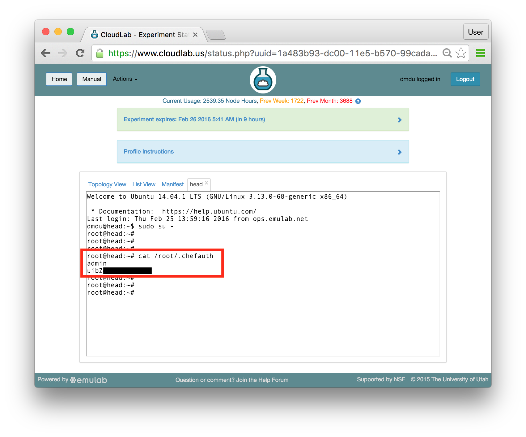
Expand the “Profile Instructions” panel and click on the “Chef web console” link.
Warning: When your browser first points to this link, you will see a warning about using a self-signed SSL certificate. Using self-signed certificates is not a good option in production scenarios, but it is totally acceptable in this short-term experimentation environment. We will ignore this warning and proceed to using the Chef console. The sequence of steps for ignoring it depends on your browser. In Chrome, you will see a message saying "Your connection is not private". Click “Advanced” at the bottom of the page and choose “Proceed to <hostname> (unsafe)”. In Firefox, the process is slightly different: click “Advanced”, choose “Add Exception”, and click “Confirm Security Exception”.
When the login page is finally displayed, use the credentials you have printed in the shell:
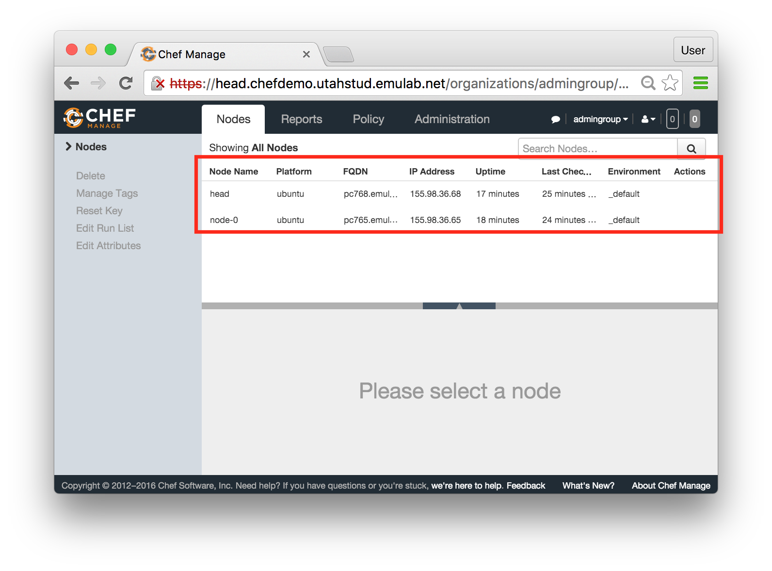
If you see a console like the one above, with both head and node-0 listed on the “Nodes” tab, you have a working Chef cluster! You can now proceed to managing your nodes using Chef recipes, cookbooks, and roles.
In the rest of the tutorial, we demonstrate how you can use several pre-defined cookbooks and roles.
Development of cookbooks and roles is a subject of another tutorial (many such tutorials can be
found online). Our goal in the following sections is to walk you through
the process of using existing cookbooks and roles —
16.9 Configuring NFS
Now that you have a working instance of Chef where both head and node-0 can be controlled using Chef, let’s start modifying the software stacks on these nodes by installing NFS and exporting a directory from head to node-0.
- Modify the run list on headClick on the row for head in the node list (so the entire row is highlighted in orange), and then click "Edit" in the Run List panel in the bottom right corner of the page:
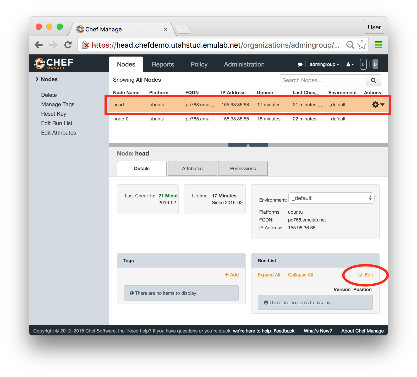
- Apply nfs role:In the popup window, find the role called nfs in the Available Roles list on the left, drag and drop it into the "Current Run List" field on the right. When this is done, click "Save Run List".
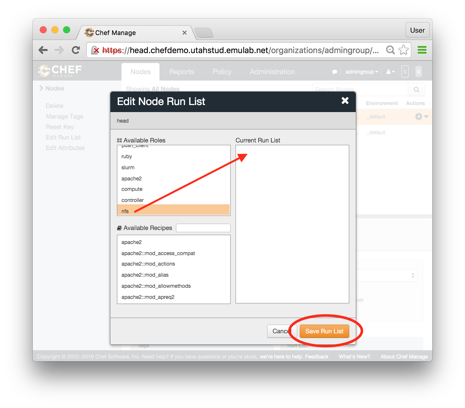
- Repeat the last two steps for node-0:
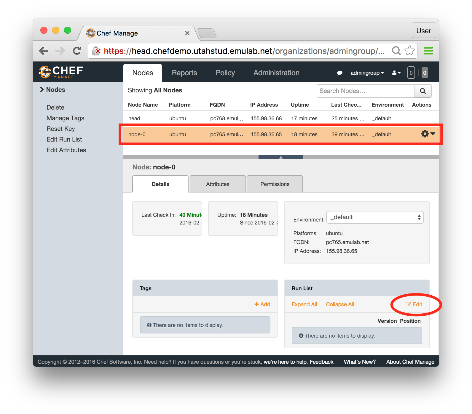
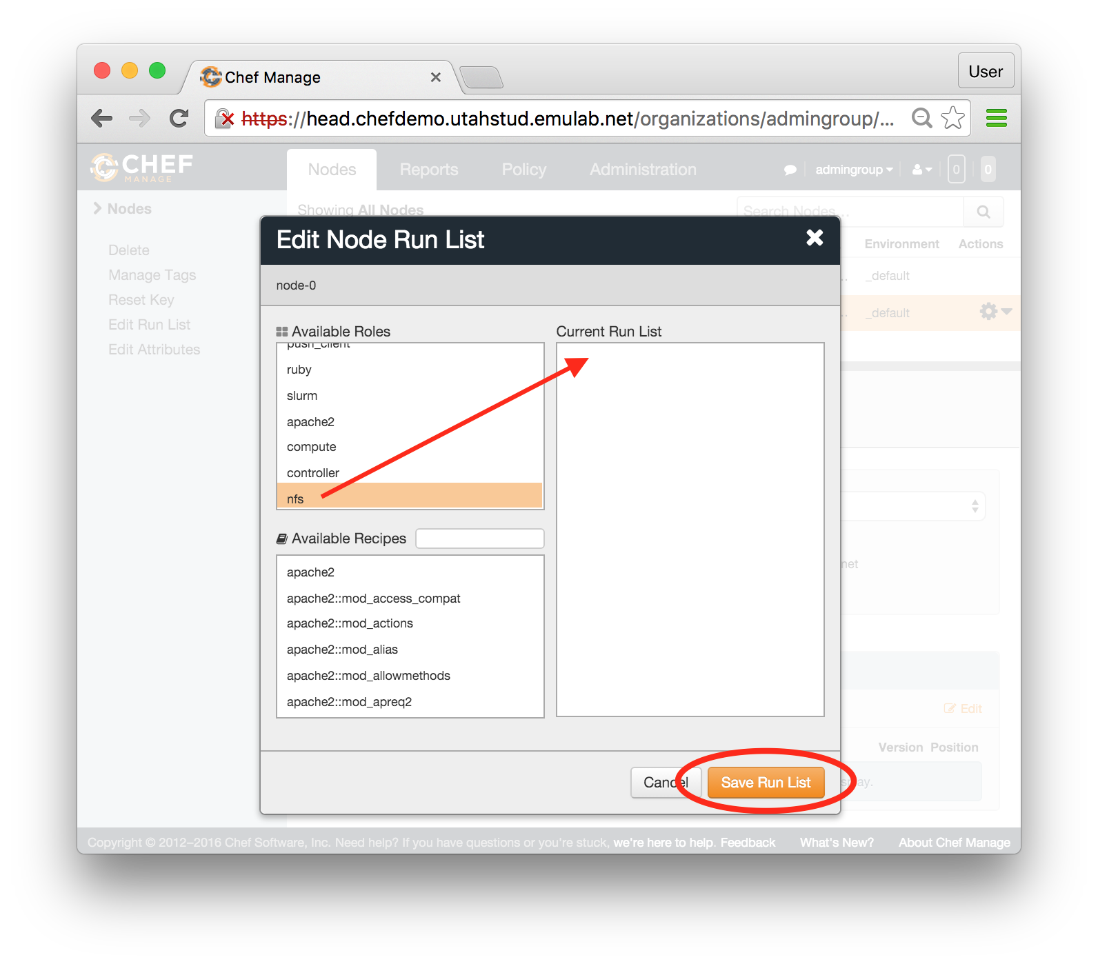 At this point, nfs role is assigned to both nodes, but nothing has executed yet.
 - Check the status from the shellBefore proceeding to applying these updates, let’s check the role assignment from the shell by typing:
knife status -r
The run lists for your nodes should be printed inside square brackets: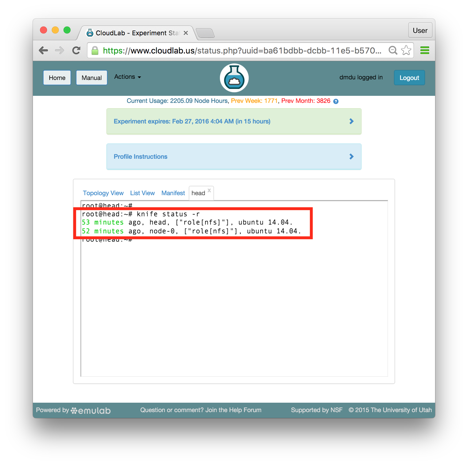 The output of this command also conveniently shows when Chef applied changes to your nodes last (first column) and what operating systems run on the nodes (last column).
 - Trigger the updatesRun the assigned role on head by typing:
chef-client
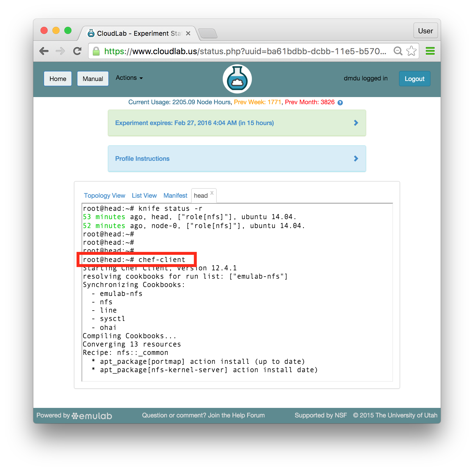 As a part of the startup procedure, passwordless ssh connections are enabled between the nodes. Therefore, you can use ssh to run commands remotely, on the nodes other than head, from the same shell. Execute the same command on node-0 by typing:
ssh node-0 chef-client
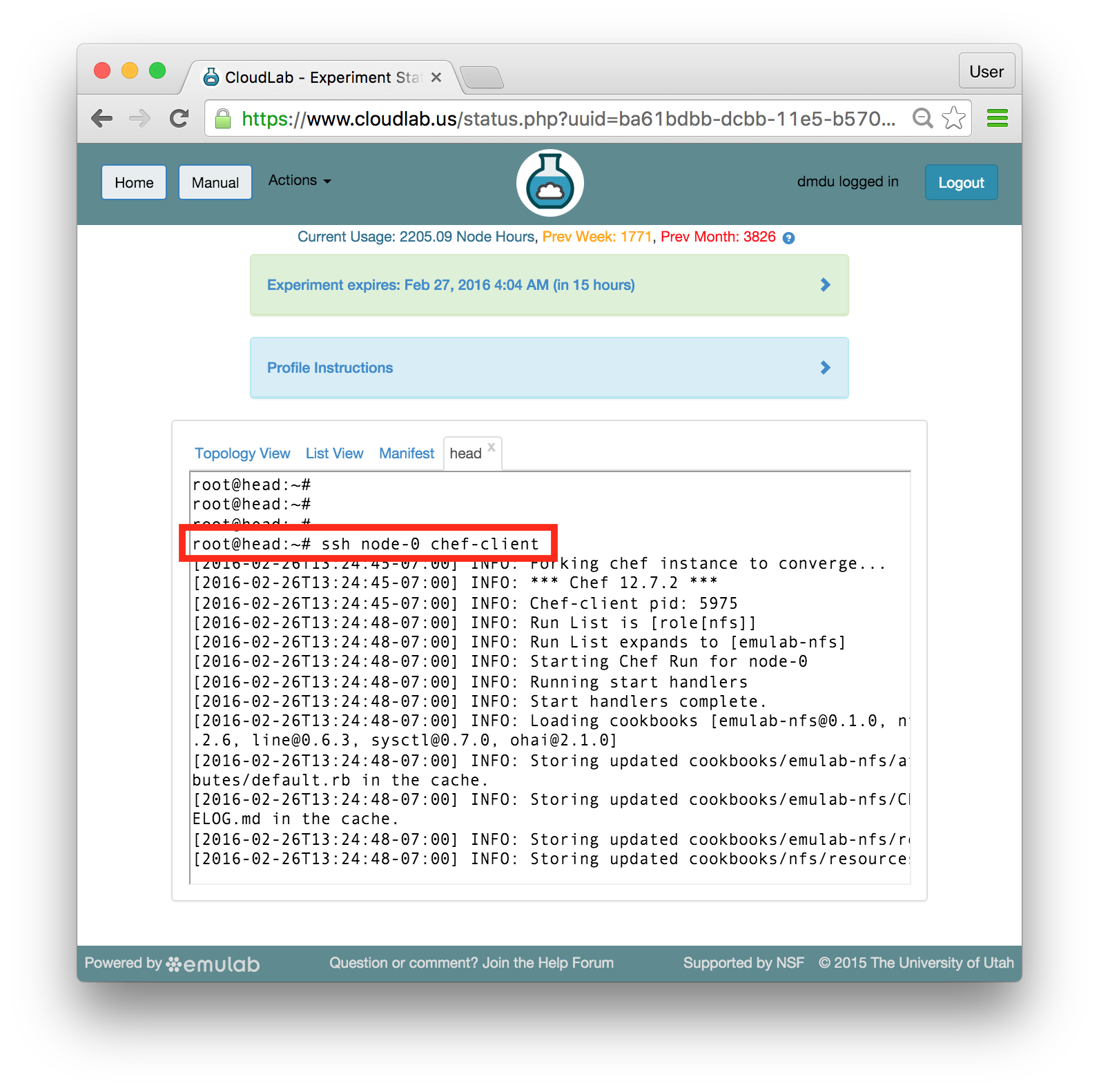 When nodes execute the “chef-client” command, they contact the server and request the cookbooks, recipes, and roles have been assigned to them in their run lists. The server responds with those artifacts, and the nodes execute them in the specified order.
 - Verify that NFS is workingAfter updating both nodes, you should have a working NFS configuration in which the /exp-share directory is exported from head and mounted on node-0.
The name of the NFS directory is one of the attributes that is set in the nfs role. To explore other attributes and see how this role is implemented, take a look at the /chef-repo/roles/nfs.rb file on head
The simplest way to test that this configuration is functioning properly is to create a file on one node and check that this file becomes available on the other node. Follow these commands to test it (the lines that start with the # sign are comments):# List files in the NFS directory /exp-share on head; should be empty
ls /exp-share/
# List the same directory remotely on node-0; also empty
ssh node-0 ls /exp-share/
# Create an empty file in this derectory locally
touch /exp-share/NFS-is-configured-by-Chef
# Find the same file on node-0
ssh node-0 ls /exp-share/
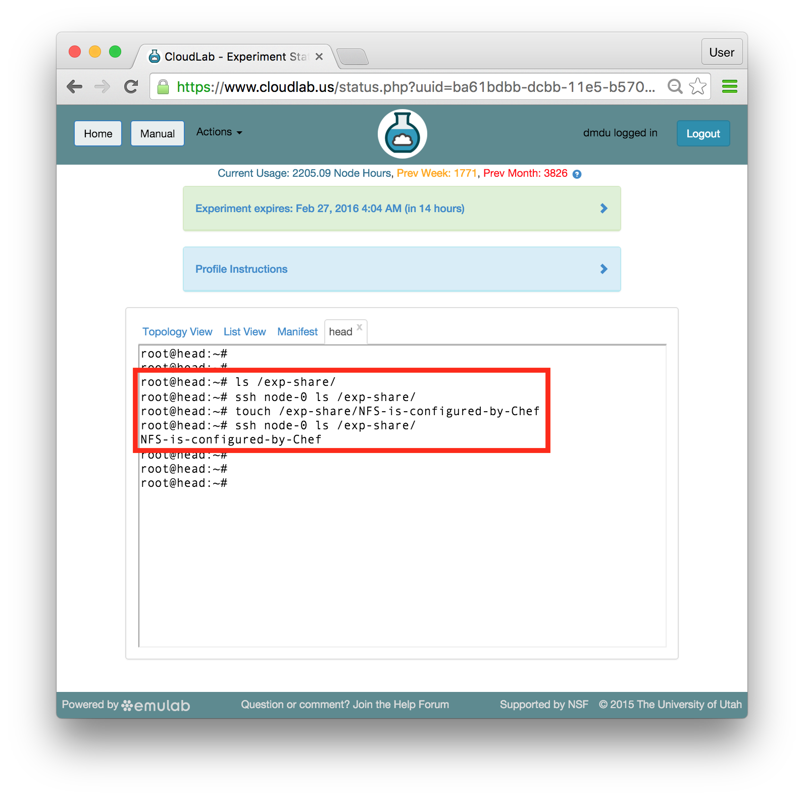 If you can see the created file on node-0, your NFS is working as expected. Now you can easily move files between your nodes using the /exp-share directory.
Summary: You have just installed and configured NFS by assigning a Chef role and running it on your nodes. You can create much more complex software environments by repeating these simple steps and installing more software components on your nodes. Additionally, installing NFS on a set of nodes is not a subject of a research experiment but rather an infrastructure prerequisite for many distributed systems. You can automate installation and configuration procedures in those systems using a system like Chef and save a lot of time when you need to periodically recreate them or create multiple instances of those systems.
16.9.1 Exploring The Structure
It is worth looking at how the role you have just used is implemented. Stored at /chef-repo/roles/nfs.rb on head, it should include the following code:
# |
# This role depends on the emulab-nfs cookbook; |
# emulab-nfs depends on the nfs cookbook |
# available at: https://supermarket.chef.io/cookbooks/nfs |
# Make sure it is installed; If it is not, try: knife cookbook site install nfs |
# |
name "nfs" |
description "Role applied to all NFS nodes - server and client" |
override_attributes( |
"nfs" => { |
"server" => "head", |
"dir" => "/exp-share", |
"export" => { |
"network" => "10.0.0.0/8", |
"writeable" => true |
} |
} |
) |
run_list [ "emulab-nfs" ] |
You can see a number of domain-specific Ruby attributes in this file. name and description are self-describing attributes. The override_attribute attribute allows you to control high-level configuration parameters, including (but not limited to) the name of the node running the NFS server, the directory being exported and mounted, the network in which this directory is shared, and the “write” permission in this directory (granted or not). The run_list attribute includes a single cookbook called emulab-nfs.
You are probably wondering now about how the same cookbook can perform different actions on different nodes. Indeed, the emulab-nfs cookbook has just installed NFS server on head and NFS client on node-0. You can take a look at the implementation of the default.rb, the default recipe in the emulab-nfs cookbook which gets called when the cookbook is executed. You should find the following code at /chef-repo/cookbooks/emulab-nfs/recipes/default.rb:
# |
# Cookbook Name:: emulab-nfs |
# Recipe:: default |
# |
|
if node["hostname"] == node["nfs"]["server"] |
include_recipe "emulab-nfs::export" |
else |
include_recipe "emulab-nfs::mount" |
end |
The if statement above allows comparing the hostname of the node on which the cookbook is running with one of the attributes specified in the role. Based on this comparison, the recipe takes the appropriate actions by calling the code from two other recipes in this cookbook. Optionally, you can explore /chef-repo/cookbooks/emulab-nfs/recipes/export.rb and /chef-repo/cookbooks/emulab-nfs/recipes/mount.rb to see how these recipes are implemented.
Obviously, this is not the only possible structure for this configuration. You can alternatively create two roles, such as nfs-server and nfs-client, that will call the corresponding recipes without the need for the described comparison. Since a single model cannot fit perfectly all scenarios, Chef provides the developer with enough flexibility to organize the code into structures that match specific environment and application needs.
16.10 Apache Web Server and ApacheBench Benchmarking tool
In this exercise, we are going to switch gears and experiment with
different software —
We recommend you to continue using the shell tab for head (again, make sure that your commands are executed as root). Run the commands described below in that shell.
- Add a role to the head’s run listIssue the command in bold (the rest is the expected output):
knife node run_list add head "role[apache2]"
head:
run_list:
role[nfs]
role[apache2]
- Add two roles to the node-0’s run listRun the two knife commands listed below (also on head) in order to assign two roles to node-0:
knife node run_list add node-0 "role[apache2]"
run_list:
head:
run_list:
role[nfs]
role[apache2]
knife node run_list add node-0 "role[apachebench]"
run_list:
head:
run_list:
role[nfs]
role[apache2]
role[apachebench]
Notice that we did not exclude the nfs role from the run lists. Configuration updates in Chef are idempotent, which means that an update can be applied to a node multiple times, and every time the update will yield identical configuration (regardless of the node’s previous state) Thus, this time, when you run “chef-client” again, Chef will do the right thing: the state of each individual component will be inspected, and all NFS-related tasks will be silently skipped because NFS is already installed. - Trigger updates on all nodesIn the previous section, we updated one node at a time. Try the “batch” update - run a single command that will trigger configuration procedures on all client nodes:
knife ssh "name:*" chef-client
apt155.apt.emulab.net resolving cookbooks for run list:
["emulab-nfs", "apache2", "apache2::mod_autoindex", "emulab-apachebench"]
apt154.apt.emulab.net resolving cookbooks for run list:
["emulab-nfs", "apache2", "apache2::mod_autoindex"]
apt155.apt.emulab.net Synchronizing Cookbooks:
....
apt155.apt.emulab.net Chef Client finished, 5/123 resources updated in 04 seconds
You should see interleaved output from the “chef-client” command running on both nodes at the same time.The last command uses a node search based on the “name:*” criteria. As a result, every node will execute “chef-client”. In cases where it is necessary, you can use more specific search strings, such as, for instance, “name:head” and “name:node-*”. - Check that the webservers are runningOne of the attributes in the apache2 role configures the web server such that it runs on the port 8080. Let’s check that the web servers are running via checking the status of that port:
knife ssh "name:*" "netstat -ntpl | grep 8080"
pc765.emulab.net tcp6 0 0 :::8080 :::* LISTEN 9415/apache2
pc768.emulab.net tcp6 0 0 :::8080 :::* LISTEN 30248/apache2
Note that this command sends an arbitrary command (unrelated to Chef) to a group of nodes. With this functionality, the knife command-line utility can be viewed as an orchestration tool for managing groups of nodes that is capable of replacing pdsh, the Parallel Distributed Shell utility, that is often used on computing clusters.The output that is similar to the one above indicates that both apache2 web servers are running. The command that you have just issued uses netstat, a command-line tool that displays network connections, routing tables, interface statistics, etc. Using knife, you have run netstat in combination with a Linux pipe and a grep command for filtering output and displaying the information only on the port 8080. - Check benchmarking results on node-0Many different actions have taken place on node-0, including:
apache2 has been installed and configured
ab, a benchmarking tool from the apache2-utils package, has been installed and executed
benchmarking results have been saved, and plots have been created using the gnuplot utility
the plots have been made available using the installed web server
To see how the last three tasks are performed using Chef, you can take a look at the default.rb recipe inside the emulab-apachebench cookbook. In the in-person tutorial, let’s proceed to the following steps and leave the discussion of this specific recipe and abstractions used in Chef recipes in general to the end of the tutorial.Obtain the node-0’s public hostname (refer to the list included in the profile instructions), and construct the following URL:http://<node-0's public hostname>:8080
With the right hostname, copy and paste this URL into your browser to access the web server running on node-0 and serving the benchmarking graphs. You should see a directory listing like this: You can explore the benchmarking graphs by clicking at the listed links. So far, ab has run against the local host (i.e. node-0), therefore the results may not be so interesting. Do not close the window with your browser since one of the following steps will ask you to go back to it to see more results.
 - Modify a roleJust like the nfs role described in the previous section, apachebench has a number of attributes that define its behavior. We will use the Chef web console to update the value for one of its attributes.In the console, click on the Policy tab at the top of the page, choose “Roles” in the panel on the left, and select “apachebench” in the displayed list of roles. Select the Attributes tab in the middle of the page. At the bottom of the page, you should now see a panel called “Override Attributes”. Click the “Edit” button inside that panel:
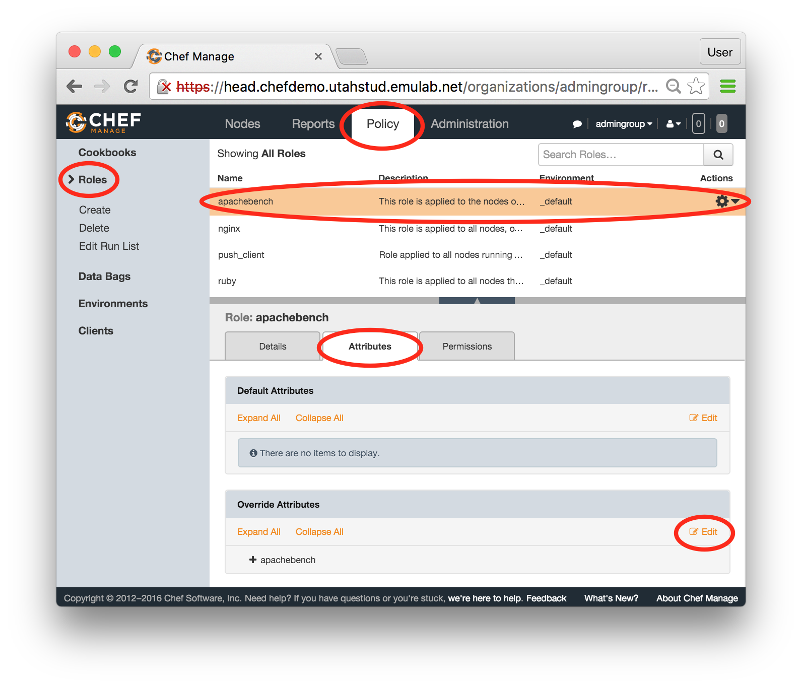 In the popup window, change the target_host attribute from null to the head’s public hostname (refer to the hostnames listed in the profile instructions). Don’t forget to use double quotes around the hostname. Also, let’s modify the list of ports against which we will run the benchmark. Change 80 to 8080 since nothing interesting is running on port 80, while the apache2 server you have just installed is listening on the port 8080. Leave the port 443 in the list —
this is the port on which the Chef web console is running. Here is an example of the recommended changes: 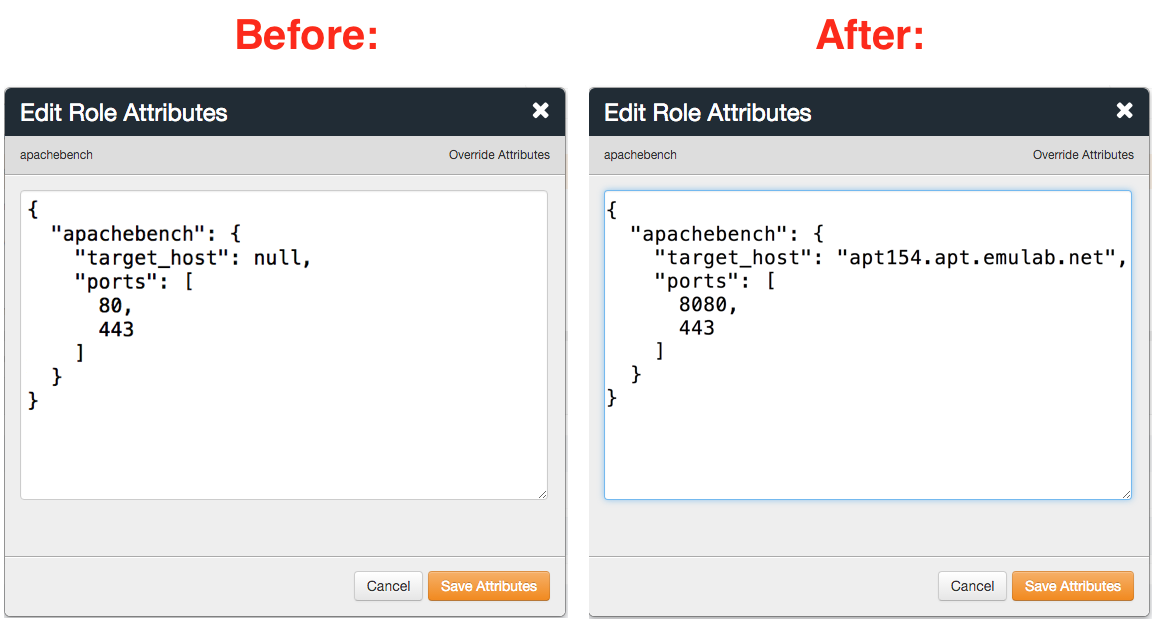 When these changes are complete, click "Save Attributes".Alternative: It turns out that you don’t have to use the Chef web console for modifying this role. Take a look at the two steps described below to see how we can modify this role from the shell or skip to running the benchmark.This is what you need to make the described changes without using the web console:
Edit the file /chef-repo/roles/apachebench.rb on head using a text editor of your choice (e.g., vi)
After making the suggested changes, “push” the updated role to the server by typing: knife role from file /chef-repo/roles/apachebench.rb
- Run the benchmark against headThe updated version of the role is available on the server now. You can run it on node-0 using the following command:
knife ssh "role:apachebench" chef-client
This command, unlike the knife commands you issued in the previous steps, uses a search based on the assigned roles. In other words, it will find the nodes to which the apachebench role has been assigned by now —in our case, only node-0 — and execute “chef-client” on them. - Check benchmarking results againGo back to your browser window and update the page to see the directory listing with new benchmarking results.
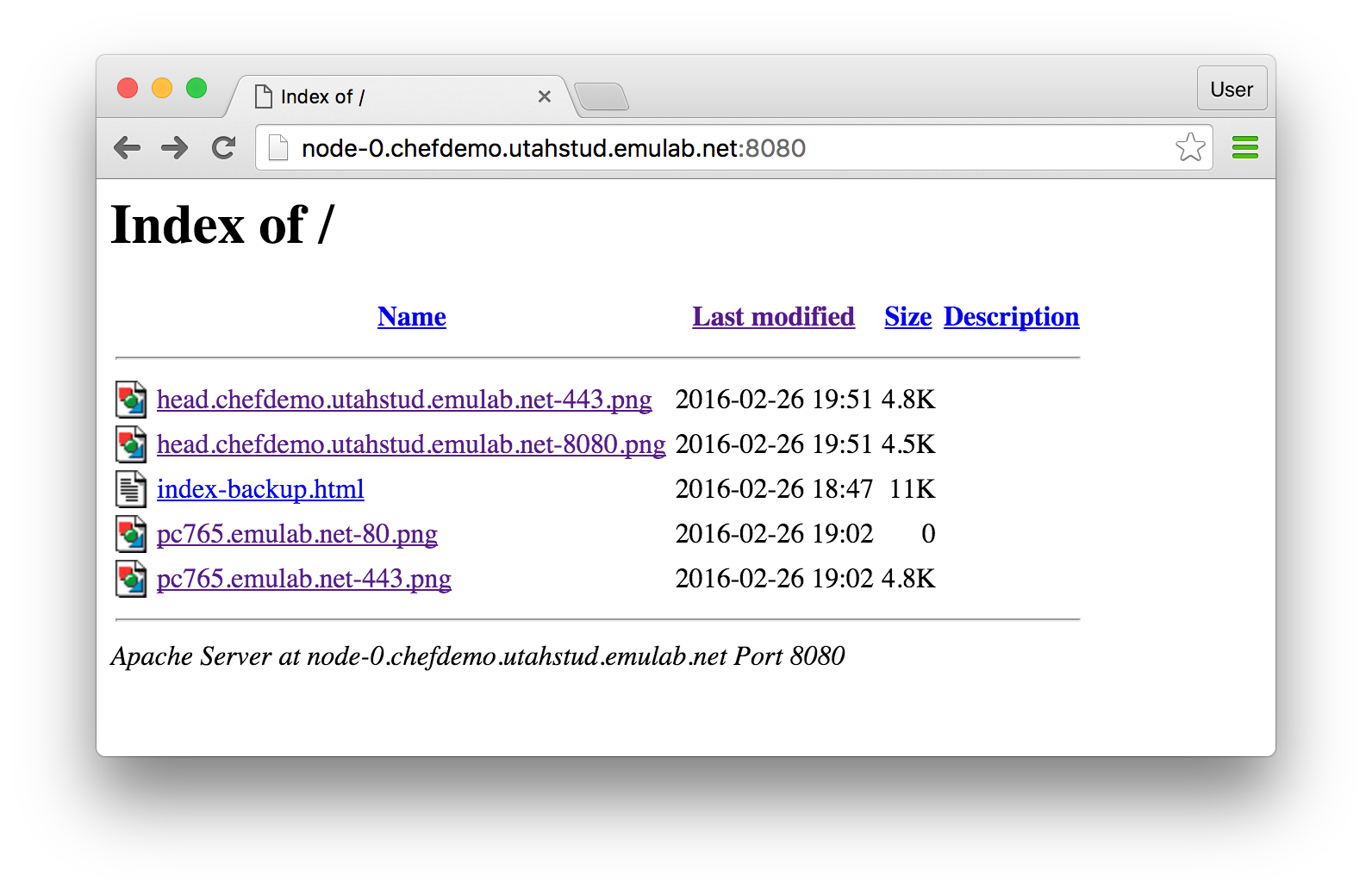 The first two (the most recent) graphs represent the results of benchmarking of the web services running on head performed from node-0. Among many interesting facts that are revealed by these graphs, you will see that the response time is much higher on the port 443 than on the port 8080.
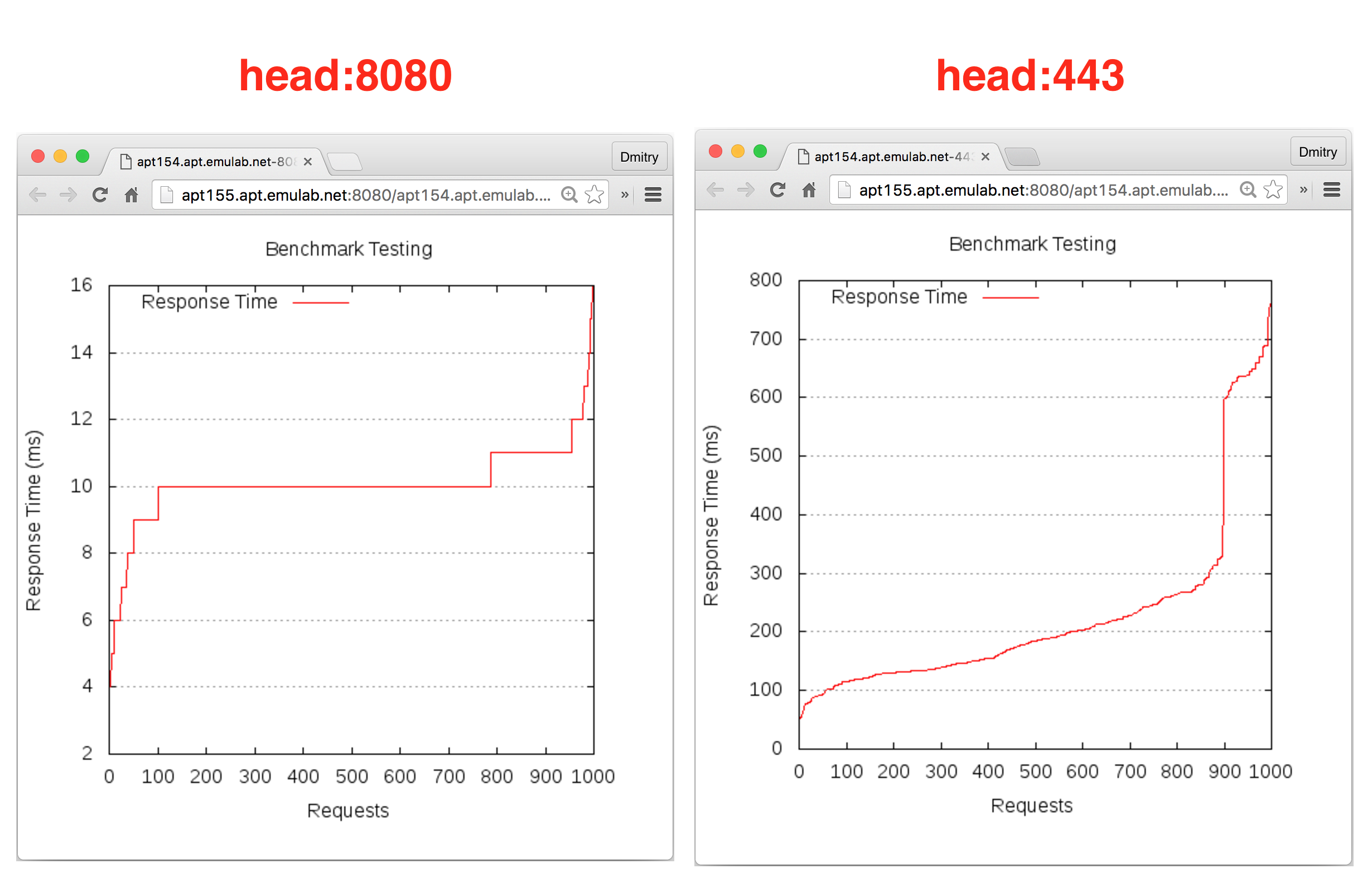
Summary: You have just performed an experiment with apache2 and ab in a very automated manner. The Chef role you have used performed many tasks, including setting up the infrastructure, running a benchmark, saving and processing results, as well as making them easily accessible. The following section will shed some light on how these tasks were accomplished and also how they can be customized.
16.10.1 Understanding the Internals
Below we describe some of the key points about the pieces of infrastructure code you have just used.
The apache2 role is stored at roles/apache2.rb as part of the emulab/chef-repo. Note that the run list specified in this role includes a cookbook apache2 (the recipe called default.rb inside the cookbook is used) and also a recipe mod_autoindex from the same cookbook. This cookbook is one of the cookbooks that have been obtained from Chef Supermarket. All administrative work for installing and configuring the web server is performed by the recipes in this cookbook, while the role demonstrates an example of how that cookbook can be “wrapped” into a specification that satisfy specific application needs.
The apachebench role is stored at roles/apachebench.rb It specifies values for several attributes and adds a custom cookbook emulab-apachebench to the run list. We use the “emulab” prefix in the names of the cookbooks that have been developed by the CloudLab staff to emphasize that they are developed for Emulab and derived testbeds such as CloudLab. This also allows distinguishing them from the Supermarket cookbooks, which are installed in the same directory on head.
Inside the default.rb recipe in emulab-apachebench you can find many key words, including package, log, file, execute, template, etc. They are called Chef resources. These elements, which allow defining fine-grained configuration tasks and actions, are available for many common administrative needs. You can refer to the list of supported Chef resources and see examples of how they can be used.
Another item that is worth mentioning is the “ignore_failure true” attribute used in some of the resources. It allows the recipe to continue execution even when something does not go as expected (shell command fail, necessary files do not exist, etc.). Also, when relying on specific files in your recipes, you can augment resources with additional checks like “only_if{::File.exists?(<file name>)}” and “not_if{::File.exists?(<file name>)}” to make your infrastructure code more reliable and repeatable (this refers to the notion of idempotent code mentioned earlier).
16.11 Final Remarks about Chef on CloudLab
In this tutorial, you had a chance to explore the Chef configuration management system and used some of its powerful features for configuration management in a multi-node experiment on CloudLab. Even though the instructions walked you through the process of configurating only two nodes, you can use the demonstrated code artifacts, such as roles, cookbooks, recipes, and resources, and apply them to infrastructure in larger experiments. With the knife commands like the ones shown above, you can “orchestrate” diverse and complex applications and environments.
When establishing such orchestration in your experiments, you can take advantage of the relevant pieces of intrastructure code, e.g., available through Chef Supermarket. In cases when you have to develop your own custom code, you may adopt the structure and the abstractions supported by Chef and aim to develop infrastructure code that is modular, flexible, and easy to use.
The ChefCluster profile is available to all users on CloudLab. If you are interested in learning more about Chef and developing custom infrastructure code for your experiments, this profile will spare you from the need to set up necessary components every time and allow you to run a fully functional Chef installation for your specific needs.
16.12 Terminating Your Experiment
Resources that you hold in CloudLab are real, physical machines and are therefore limited and in high demand. When you are done, you should release them for use by other experimenters. Do this via the “Terminate” button on the CloudLab experiment status page.
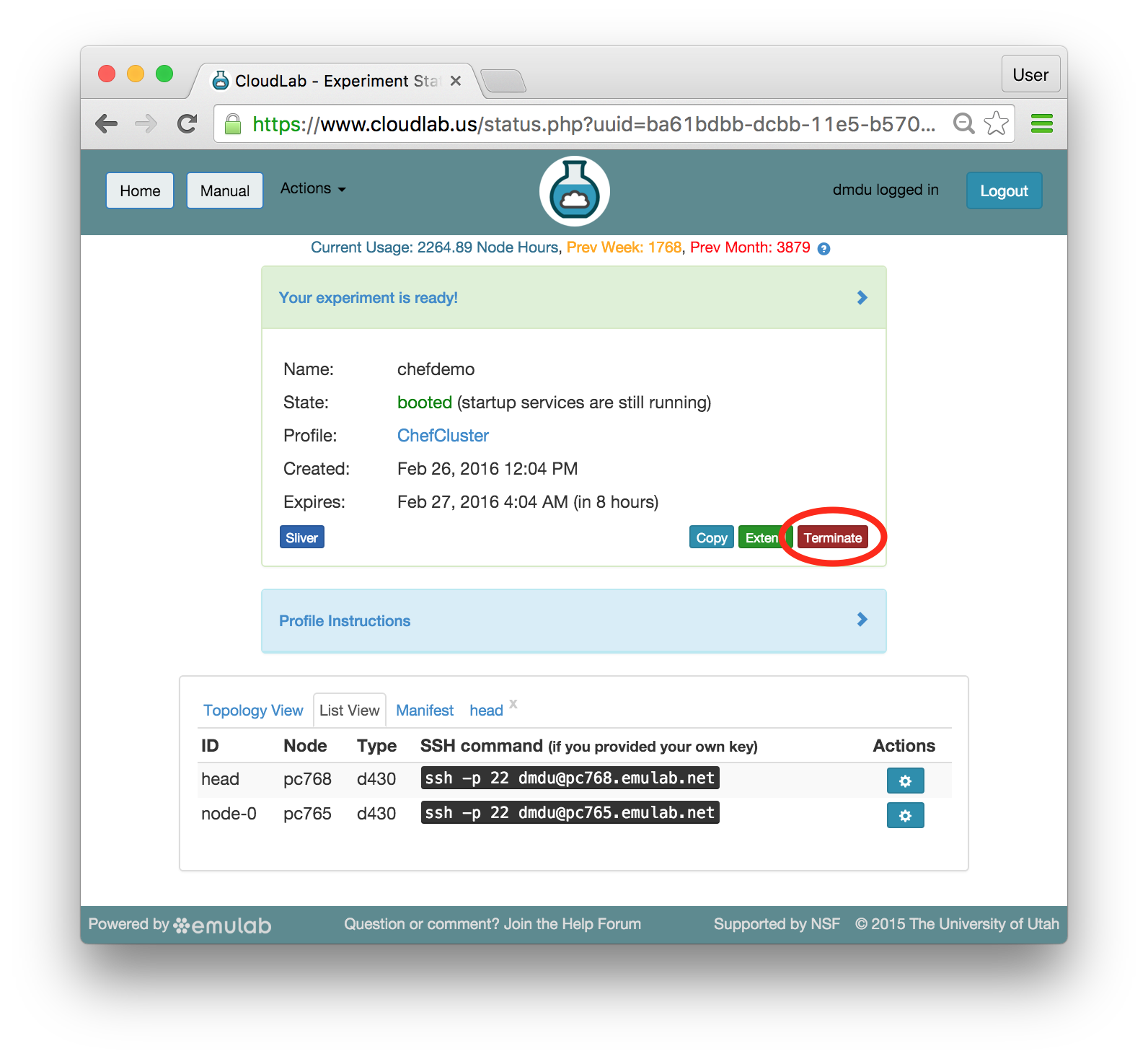
Note: When you terminate an experiment, all data on the nodes is lost, so make sure to copy off any data you may need before terminating.
If you were doing a real experiment, you might need to hold onto the nodes for longer than the default expiration time. You would request more time by using the “Extend” button the on the status page. You would need to provide a written justification for holding onto your resources for a longer period of time.
16.13 Future Steps
Now that you’ve got a feel for how Chef can help manage experiment resources, there are several things you might try next:
Learn more about Chef at the Chef official website
Explore existing cookbooks and roles in the emulab/chef-repo repository
Follow the steps in the Guide to Writing Chef Cookbooks blog post by Joshua Timberman, a Chef developer and one of the active members of the Chef community
Configure a LAMP (Linux, Apache, MySql, and PHP) stack using Chef by following the Creating Your First Chef Cookbook tutorial
17 Citing CloudLab
If you use CloudLab in an academic publication, we ask that you refer to it by name in your text, and that you cite the paper below: it helps us find papers that have used the facility, helps readers know about the environment in which your experiments were run, and helps us to report on the testbed’s use to our funders.
Thanks!
@inproceedings{Duplyakin+:ATC19, |
title = "The Design and Operation of {CloudLab}", |
author = "Dmitry Duplyakin and Robert Ricci and Aleksander Maricq and Gary Wong and Jonathon Duerig and Eric Eide and Leigh Stoller and Mike Hibler and David Johnson and Kirk Webb and Aditya Akella and Kuangching Wang and Glenn Ricart and Larry Landweber and Chip Elliott and Michael Zink and Emmanuel Cecchet and Snigdhaswin Kar and Prabodh Mishra", |
booktitle = "Proceedings of the {USENIX} Annual Technical Conference (ATC)", |
pages = "1--14", |
year = 2019, |
month = jul, |
url = "https://www.flux.utah.edu/paper/duplyakin-atc19" |
} |
|
18 Getting Help
The help forum is the main place to ask questions about CloudLab, its use, its default profiles, etc. Users are strongly encouraged to participate in answering other users’ questions. The help forum is handled through Google Groups, which, by default, sends all messages to the group to your email address. You may change your settings to receive only digests, or to turn email off completely.
The forum is searchable, and we recommend doing a search before asking a question.
The URL for joining or searching the forum is: https://groups.google.com/forum/#!forum/cloudlab-users
If you have any questions that you do not think are suitable for a public forum, you may direct them to support@cloudlab.us